Universal Non-Uniform Random Number Sampling in SciPy#
SciPy provides an interface to many universal non-uniform random number generators to sample random variates from a wide variety of univariate continuous and discrete distributions. Implementations of a fast C library called UNU.RAN are used for speed and performance. Please look at UNU.RAN’s documentation for an in-depth explanation of these methods. It is heavily referred to for writing this tutorial and the documentation of all the generators.
Introduction#
Random variate generation is the small field of research that deals with algorithms to generate random variates from various distributions. It is common to assume that a uniform random number generator is available. This is a program that produces a sequence of independent and identically distributed continuous \(U(0,1)\) random variates (i.e. uniform random variates on the interval \((0,1)\)). Of course, real-world computers can never generate ideal random numbers and they cannot produce numbers of arbitrary precision but state-of-the-art uniform random number generators come close to this aim. Thus, random variate generation deals with the problem of transforming such a sequence of \(U(0,1)\) random numbers into non-uniform random variates. These methods are universal and work in a black-box fashion.
Some methods to do that are:
The Inversion method: When the inverse \(F^{-1}\) of the cumulative distribution function is known, then random variate generation is easy. We just generate a uniformly \(U(0,1)\) distributed random number U and return \(X = F^{-1}(U)\). As closed form solutions for the inverse are rarely available, one usually needs to rely on approximations of the inverse (e.g.
scipy.special.ndtri,scipy.special.stdtrit). In general, the implementation of special functions is quite slow compared to the inversion methods in UNU.RAN.The Rejection Method: The rejection method, often called acceptance-rejection method, has been suggested by John von Neumann in 1951[1]. It involves computing an upper bound to the PDF (also called the hat function) and using the inversion method to generate a random variate, say \(Y\), from this bound. Then a uniform random number can be drawn between \(0\) and the value of the upper bound at \(Y\). If this number is less than the PDF at \(Y\), return the sample otherwise reject it. See
scipy.stats.sampling.TransformedDensityRejection.The Ratio-of-Uniforms Method: This is a type of acceptance-rejection method which is uses minimal bounding rectangles to construct the hat function. See
scipy.stats.sampling.RatioUniforms.Inversion for Discrete Distributions: The difference compared to the continuous case is that \(F\) is now a step-function. To realize this in a computer, a search algorithm is used, the simplest of which is sequential search. A uniform random number is generated from \(U(0, 1)\) and probabilities are summed until the cumulative probability exceeds the uniform random number. The index at which this happens is the required random variate and is returned.
More details on these algorithms can be found in the appendix of the UNU.RAN user manual.
When generating random variates of a distribution, two factors are important to determine the speed of a generator: the setup step and the actual sampling. Depending on the situation, different generators can be optimal. For example, if one repeatedly needs to draw large samples from a given distribution with a fixed shape parameter, a slow setup is acceptable if the sampling is fast. This is called the fixed parameter case. If one aims to generate samples of a distribution for different shape parameters (the varying parameter case), an expensive setup that needs to be repeated for each parameter would lead to very poor performance. In such a situation, a fast setup is crucial to achieve good performance. An overview of the setup and sampling speed of the different methods is shown in the table below.
Methods for continuous distributions |
Required Inputs |
Optional Inputs |
Setup Speed |
Sampling Speed |
|---|---|---|---|---|
pdf, dpdf |
none |
slow |
fast |
|
cdf |
pdf, dpdf |
(very) slow |
(very) fast |
|
cdf |
(very) slow |
(very) fast |
||
none |
fast |
slow |
where
pdf: probability density function
dpdf: derivative of the pdf
cdf: cumulative distribution function
To apply the numerical inversion method NumericalInversePolynomial to a large
number of continuous distributions in SciPy with minimal effort, take a look
at scipy.stats.sampling.FastGeneratorInversion.
Methods for discrete distributions |
Required Inputs |
Optional Inputs |
Setup Speed |
Sampling Speed |
|---|---|---|---|---|
pv |
pmf |
slow |
very fast |
|
pv |
pmf |
slow |
very fast |
where
pv: probability vector
pmf: probability mass function
For more details on the generators implemented in UNU.RAN, please refer to [2] and [3].
Basic concepts of the Interface#
Every generator needs to be set up before one can start sampling from it.
This can be done by instantiating an object of that class. Most of the
generators take a distribution object as input which contains the implementation
of required methods like PDF, CDF, etc. In addition to the distribution
object, one can also pass parameters used to set up the generator. It is also
possible to truncate the distributions using a domain parameter. All
generators need a stream of uniform random numbers that are transformed into
random variates of the given distribution. This is done by passing a random_state
parameter with a NumPy BitGenerator as the uniform random number generator.
random_state can either be an integer, numpy.random.Generator,
or numpy.random.RandomState.
Warning
Use of NumPy < 1.19.0 is discouraged as it doesn’t have a fast Cython API for generating uniform random numbers and might be too slow for practical use.
All the generators have a common rvs method that can be used to draw
samples from the given distribution.
An example of this interface is shown below:
from scipy.stats.sampling import TransformedDensityRejection
from math import exp
import numpy as np

class StandardNormal:
    def pdf(self, x: float) -> float:
        # note that the normalization constant isn't required
        return exp(-0.5 * x*x)
    def dpdf(self, x: float) -> float:
        return -x * exp(-0.5 * x*x)

dist = StandardNormal()
urng = np.random.default_rng()
rng = TransformedDensityRejection(dist, random_state=urng)
As shown in the example, we first initialize a distribution object that
contains an implementation of the methods required by the generator. In
our case, we use the TransformedDensityRejection (TDR)
method which requires a PDF and its derivative w.r.t. x (i.e. the variate).
Note
Note that the methods of the distribution (i.e. pdf, dpdf, etc) need not
be vectorized. They should accept and return floats.
Note
One can also pass the SciPy distributions as arguments. However, note that the
object doesn’t always have all the information required by some generators
like the derivative of PDF for the TDR method. Relying on SciPy distributions
might also reduce performance due to the vectorization of the methods like
pdf and cdf. In both cases, one can implement a custom distribution object
that contains all the required methods and that is not vectorized as shown in
the example above. If one wants to apply a numerical inversion method to a
distribution defined in SciPy, please also take a look at
scipy.stats.sampling.FastGeneratorInversion.
In the above example, we have set up an object of the
TransformedDensityRejection method to sample from a
standard normal distribution. Now, we can start sampling from our
distribution by calling the rvs method:
rng.rvs()
-0.08519190405786464
rng.rvs((5, 3))
array([[-1.46666546,  0.95046314,  0.81645618],
       [ 0.09461853, -0.30302203,  2.42620421],
       [-0.13662934,  0.18591511, -1.0127185 ],
       [ 0.35013987, -0.57230565,  0.19929616],
       [-0.20122886, -0.48941685,  2.81766146]])
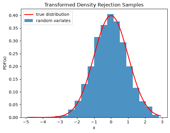
We can also check that the samples are drawn from the correct distribution by visualizing the histogram of the samples:
import numpy as np
import matplotlib.pyplot as plt
from scipy.stats import norm
from scipy.stats.sampling import TransformedDensityRejection
from math import exp

class StandardNormal:
    def pdf(self, x: float) -> float:
        # note that the normalization constant isn't required
        return exp(-0.5 * x*x)
    def dpdf(self, x: float) -> float:
        return -x * exp(-0.5 * x*x)

dist = StandardNormal()
urng = np.random.default_rng()
rng = TransformedDensityRejection(dist, random_state=urng)
rvs = rng.rvs(size=1000)
x = np.linspace(rvs.min()-0.1, rvs.max()+0.1, num=1000)
fx = norm.pdf(x)
plt.plot(x, fx, 'r-', lw=2, label='true distribution')
plt.hist(rvs, bins=20, density=True, alpha=0.8, label='random variates')
plt.xlabel('x')
plt.ylabel('PDF(x)')
plt.title('Transformed Density Rejection Samples')
plt.legend()
plt.show()
Note
Please note the difference between the rvs method of the distributions
present in scipy.stats and the one provided by these generators.
UNU.RAN generators must be considered independent in a sense that they will
generally produce a different stream of random numbers than the one produced
by the equivalent distribution in scipy.stats for any seed. The
implementation of rvs in scipy.stats.rv_continuous usually relies
on the NumPy module numpy.random for well-known distributions (e.g.,
for the normal distribution, the beta distribution) and transformations of
other distributions (e.g., normal inverse Gaussian
scipy.stats.norminvgauss and the lognormal
scipy.stats.lognorm distribution). If no specific method is
implemented, scipy.stats.rv_continuous defaults to a numerical
inversion method of the CDF that is very slow. As UNU.RAN transforms uniform
random numbers differently than SciPy or NumPy, the resulting stream of RVs is
different even for the same stream of uniform random numbers. For example, the
random number stream of SciPy’s scipy.stats.norm and UNU.RAN’s
TransformedDensityRejection would not be the same
even for the same random_state:
  from scipy.stats.sampling import norm, TransformedDensityRejection
  from copy import copy
  dist = StandardNormal()
  urng1 = np.random.default_rng()
  urng1_copy = copy(urng1)
  rng = TransformedDensityRejection(dist, random_state=urng1)
  rng.rvs()
  # -1.526829048388144
  norm.rvs(random_state=urng1_copy)
  # 1.3194816698862635
We can pass a domain parameter to truncate the distribution:
rng = TransformedDensityRejection(dist, domain=(-1, 1), random_state=urng)
rng.rvs((5, 3))
array([[-0.42075748, -0.83751733,  0.92928314],
       [-0.26870526,  0.00555546, -0.43092943],
       [-0.34052945, -0.25794959, -0.72245341],
       [ 0.43809236, -0.31889987, -0.0419768 ],
       [ 0.1470709 ,  0.24549431, -0.77908996]])
Invalid and bad arguments are handled either by SciPy or by UNU.RAN. The
latter throws a UNURANError that follows a common format:
UNURANError: [objid: <object id>] <error code>: <reason> => <type of error>
where:
<object id>is the ID of the object given by UNU.RAN<error code>is an error code representing a type of error.<reason>is the reason why the error occurred.<type of error>is a short description of the type of error.
The <reason> shows what caused the error. This, by itself, should contain
enough information to help debug the error. In addition, <error id> and
<type of error> can be used to investigate different classes of error in
UNU.RAN. A complete list of all the error codes and their descriptions can be
found in the Section 8.4 of the UNU.RAN user
manual.
An example of an error generated by UNU.RAN is shown below:
UNURANError: [objid: TDR.003] 50 : PDF(x) < 0.! => (generator) (possible) invalid data
This shows that UNU.RAN failed to initialize an object with ID TDR.003
because the PDF was < 0. i.e. negative. This falls under the type
“possible invalid data for the generator” and has error code 50.
Warnings thrown by UNU.RAN also follow the same format.