scipy.stats.circvar#

scipy.stats.circvar(samples, high=6.283185307179586, low=0, axis=None, nan_policy='propagate', *, keepdims=False)[source]#

Compute the circular variance for samples assumed to be in a range.

Parameters:

samplesarray_like

Input array.

highfloat or int, optional

High boundary for the sample range. Default is 2*pi.

lowfloat or int, optional

Low boundary for the sample range. Default is 0.

axisint or None, default: None

If an int, the axis of the input along which to compute the statistic. The statistic of each axis-slice (e.g. row) of the input will appear in a corresponding element of the output. If None, the input will be raveled before computing the statistic.

nan_policy{‘propagate’, ‘omit’, ‘raise’}

Defines how to handle input NaNs.

propagate: if a NaN is present in the axis slice (e.g. row) along which the statistic is computed, the corresponding entry of the output will be NaN.
omit: NaNs will be omitted when performing the calculation. If insufficient data remains in the axis slice along which the statistic is computed, the corresponding entry of the output will be NaN.
raise: if a NaN is present, a ValueError will be raised.

keepdimsbool, default: False

If this is set to True, the axes which are reduced are left in the result as dimensions with size one. With this option, the result will broadcast correctly against the input array.

Returns:

circvarfloat: Circular variance.

See also

circmean: Circular mean.
circstd: Circular standard deviation.

Notes

This uses the following definition of circular variance: 1-R, where R is the mean resultant vector. The returned value is in the range [0, 1], 0 standing for no variance, and 1 for a large variance. In the limit of small angles, this value is similar to half the ‘linear’ variance.

Beginning in SciPy 1.9, np.matrix inputs (not recommended for new code) are converted to np.ndarray before the calculation is performed. In this case, the output will be a scalar or np.ndarray of appropriate shape rather than a 2D np.matrix. Similarly, while masked elements of masked arrays are ignored, the output will be a scalar or np.ndarray rather than a masked array with mask=False.

References

[1]

Fisher, N.I. Statistical analysis of circular data. Cambridge University Press, 1993.

Examples

>>> import numpy as np
>>> from scipy.stats import circvar
>>> import matplotlib.pyplot as plt
>>> samples_1 = np.array([0.072, -0.158, 0.077, 0.108, 0.286,
...                       0.133, -0.473, -0.001, -0.348, 0.131])
>>> samples_2 = np.array([0.111, -0.879, 0.078, 0.733, 0.421,
...                       0.104, -0.136, -0.867,  0.012,  0.105])
>>> circvar_1 = circvar(samples_1)
>>> circvar_2 = circvar(samples_2)

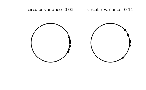
Plot the samples.

>>> fig, (left, right) = plt.subplots(ncols=2)
>>> for image in (left, right):
...     image.plot(np.cos(np.linspace(0, 2*np.pi, 500)),
...                np.sin(np.linspace(0, 2*np.pi, 500)),
...                c='k')
...     image.axis('equal')
...     image.axis('off')
>>> left.scatter(np.cos(samples_1), np.sin(samples_1), c='k', s=15)
>>> left.set_title(f"circular variance: {np.round(circvar_1, 2)!r}")
>>> right.scatter(np.cos(samples_2), np.sin(samples_2), c='k', s=15)
>>> right.set_title(f"circular variance: {np.round(circvar_2, 2)!r}")
>>> plt.show()