scipy.special.voigt_profile#

scipy.special.voigt_profile(x, sigma, gamma, out=None) = <ufunc 'voigt_profile'>#

Voigt profile.

The Voigt profile is a convolution of a 1-D Normal distribution with standard deviation sigma and a 1-D Cauchy distribution with half-width at half-maximum gamma.

If sigma = 0, PDF of Cauchy distribution is returned. Conversely, if gamma = 0, PDF of Normal distribution is returned. If sigma = gamma = 0, the return value is Inf for x = 0, and 0 for all other x.

Parameters:

xarray_like: Real argument
sigmaarray_like: The standard deviation of the Normal distribution part
gammaarray_like: The half-width at half-maximum of the Cauchy distribution part
outndarray, optional: Optional output array for the function values

Returns:

scalar or ndarray: The Voigt profile at the given arguments

See also

wofz: Faddeeva function

Notes

It can be expressed in terms of Faddeeva function

\[V(x; \sigma, \gamma) = \frac{Re[w(z)]}{\sigma\sqrt{2\pi}},\]

\[z = \frac{x + i\gamma}{\sqrt{2}\sigma}\]

where \(w(z)\) is the Faddeeva function.

References

[1]

https://en.wikipedia.org/wiki/Voigt_profile

Examples

Calculate the function at point 2 for sigma=1 and gamma=1.

>>> from scipy.special import voigt_profile
>>> import numpy as np
>>> import matplotlib.pyplot as plt
>>> voigt_profile(2, 1., 1.)
0.09071519942627544

Calculate the function at several points by providing a NumPy array for x.

>>> values = np.array([-2., 0., 5])
>>> voigt_profile(values, 1., 1.)
array([0.0907152 , 0.20870928, 0.01388492])

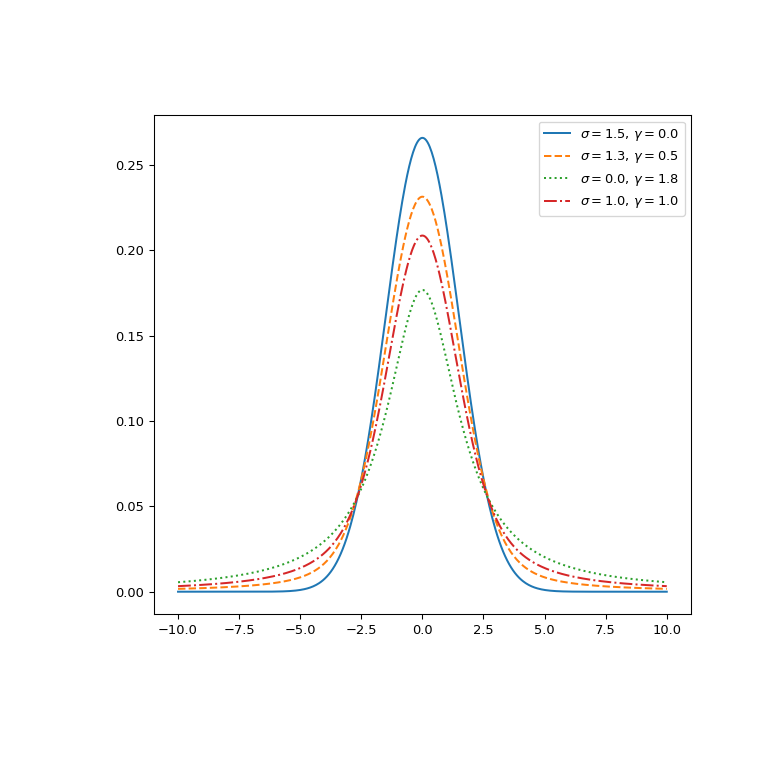
Plot the function for different parameter sets.

>>> fig, ax = plt.subplots(figsize=(8, 8))
>>> x = np.linspace(-10, 10, 500)
>>> parameters_list = [(1.5, 0., "solid"), (1.3, 0.5, "dashed"),
...                    (0., 1.8, "dotted"), (1., 1., "dashdot")]
>>> for params in parameters_list:
...     sigma, gamma, linestyle = params
...     voigt = voigt_profile(x, sigma, gamma)
...     ax.plot(x, voigt, label=rf"$\sigma={sigma},\, \gamma={gamma}$",
...             ls=linestyle)
>>> ax.legend()
>>> plt.show()

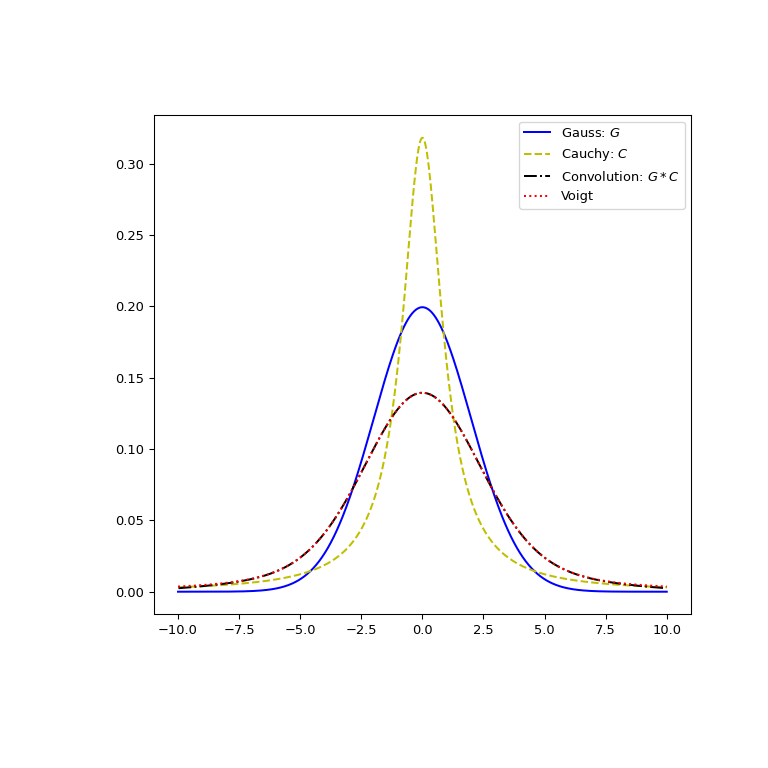
Verify visually that the Voigt profile indeed arises as the convolution of a normal and a Cauchy distribution.

>>> from scipy.signal import convolve
>>> x, dx = np.linspace(-10, 10, 500, retstep=True)
>>> def gaussian(x, sigma):
...     return np.exp(-0.5 * x**2/sigma**2)/(sigma * np.sqrt(2*np.pi))
>>> def cauchy(x, gamma):
...     return gamma/(np.pi * (np.square(x)+gamma**2))
>>> sigma = 2
>>> gamma = 1
>>> gauss_profile = gaussian(x, sigma)
>>> cauchy_profile = cauchy(x, gamma)
>>> convolved = dx * convolve(cauchy_profile, gauss_profile, mode="same")
>>> voigt = voigt_profile(x, sigma, gamma)
>>> fig, ax = plt.subplots(figsize=(8, 8))
>>> ax.plot(x, gauss_profile, label="Gauss: $G$", c='b')
>>> ax.plot(x, cauchy_profile, label="Cauchy: $C$", c='y', ls="dashed")
>>> xx = 0.5*(x[1:] + x[:-1])  # midpoints
>>> ax.plot(xx, convolved[1:], label="Convolution: $G * C$", ls='dashdot',
...         c='k')
>>> ax.plot(x, voigt, label="Voigt", ls='dotted', c='r')
>>> ax.legend()
>>> plt.show()