scipy.signal.ShortTimeFFT#

class scipy.signal.ShortTimeFFT(win, hop, fs, *, fft_mode='onesided', mfft=None, dual_win=None, scale_to=None, phase_shift=0)[source]#

Provide a parametrized discrete Short-time Fourier transform (stft) and its inverse (istft).

The stft calculates sequential FFTs by sliding a window (win) over an input signal by hop increments. It can be used to quantify the change of the spectrum over time.

The stft is represented by a complex-valued matrix S[q,p] where the p-th column represents an FFT with the window centered at the time t[p] = p * delta_t = p * hop * T where T is the sampling interval of the input signal. The q-th row represents the values at the frequency f[q] = q * delta_f with delta_f = 1 / (mfft * T) being the bin width of the FFT.

The inverse STFT istft is calculated by reversing the steps of the STFT: Take the IFFT of the p-th slice of S[q,p] and multiply the result with the so-called dual window (see dual_win). Shift the result by p * delta_t and add the result to previous shifted results to reconstruct the signal. If only the dual window is known and the STFT is invertible, from_dual can be used to instantiate this class.

Due to the convention of time t = 0 being at the first sample of the input signal, the STFT values typically have negative time slots. Hence, negative indexes like p_min or k_min do not indicate counting backwards from an array’s end like in standard Python indexing but being left of t = 0.

More detailed information can be found in the Short-Time Fourier Transform section of the SciPy User Guide.

Note that all parameters of the initializer, except scale_to (which uses scaling) have identical named attributes.

Parameters:

winnp.ndarray: The window must be a real- or complex-valued 1d array.
hopint: The increment in samples, by which the window is shifted in each step.
fsfloat: Sampling frequency of input signal and window. Its relation to the sampling interval T is T = 1 / fs.
fft_mode‘twosided’, ‘centered’, ‘onesided’, ‘onesided2X’: Mode of FFT to be used (default ‘onesided’). See property fft_mode for details.
mfft: int | None: Length of the FFT used, if a zero padded FFT is desired. If None (default), the length of the window win is used.
dual_winnp.ndarray | None: The dual window of win. If set to None, it is calculated if needed.
scale_to‘magnitude’, ‘psd’ | None: If not None (default) the window function is scaled, so each STFT column represents either a ‘magnitude’ or a power spectral density (‘psd’) spectrum. This parameter sets the property scaling to the same value. See method scale_to for details.
phase_shiftint | None: If set, add a linear phase phase_shift / mfft * f to each frequency f. The default value 0 ensures that there is no phase shift on the zeroth slice (in which t=0 is centered). See property phase_shift for more details.

Examples

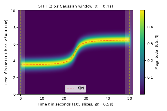
The following example shows the magnitude of the STFT of a sine with varying frequency \(f_i(t)\) (marked by a red dashed line in the plot):

>>> import numpy as np
>>> import matplotlib.pyplot as plt
>>> from scipy.signal import ShortTimeFFT
>>> from scipy.signal.windows import gaussian
...
>>> T_x, N = 1 / 20, 1000  # 20 Hz sampling rate for 50 s signal
>>> t_x = np.arange(N) * T_x  # time indexes for signal
>>> f_i = 1 * np.arctan((t_x - t_x[N // 2]) / 2) + 5  # varying frequency
>>> x = np.sin(2*np.pi*np.cumsum(f_i)*T_x) # the signal

The utilized Gaussian window is 50 samples or 2.5 s long. The parameter mfft=200 in ShortTimeFFT causes the spectrum to be oversampled by a factor of 4:

>>> g_std = 8  # standard deviation for Gaussian window in samples
>>> w = gaussian(50, std=g_std, sym=True)  # symmetric Gaussian window
>>> SFT = ShortTimeFFT(w, hop=10, fs=1/T_x, mfft=200, scale_to='magnitude')
>>> Sx = SFT.stft(x)  # perform the STFT

In the plot, the time extent of the signal x is marked by vertical dashed lines. Note that the SFT produces values outside the time range of x. The shaded areas on the left and the right indicate border effects caused by the window slices in that area not fully being inside time range of x:

>>> fig1, ax1 = plt.subplots(figsize=(6., 4.))  # enlarge plot a bit
>>> t_lo, t_hi = SFT.extent(N)[:2]  # time range of plot
>>> ax1.set_title(rf"STFT ({SFT.m_num*SFT.T:g}$\,s$ Gaussian window, " +
...               rf"$\sigma_t={g_std*SFT.T}\,$s)")
>>> ax1.set(xlabel=f"Time $t$ in seconds ({SFT.p_num(N)} slices, " +
...                rf"$\Delta t = {SFT.delta_t:g}\,$s)",
...         ylabel=f"Freq. $f$ in Hz ({SFT.f_pts} bins, " +
...                rf"$\Delta f = {SFT.delta_f:g}\,$Hz)",
...         xlim=(t_lo, t_hi))
...
>>> im1 = ax1.imshow(abs(Sx), origin='lower', aspect='auto',
...                  extent=SFT.extent(N), cmap='viridis')
>>> ax1.plot(t_x, f_i, 'r--', alpha=.5, label='$f_i(t)$')
>>> fig1.colorbar(im1, label="Magnitude $|S_x(t, f)|$")
...
>>> # Shade areas where window slices stick out to the side:
>>> for t0_, t1_ in [(t_lo, SFT.lower_border_end[0] * SFT.T),
...                  (SFT.upper_border_begin(N)[0] * SFT.T, t_hi)]:
...     ax1.axvspan(t0_, t1_, color='w', linewidth=0, alpha=.2)
>>> for t_ in [0, N * SFT.T]:  # mark signal borders with vertical line:
...     ax1.axvline(t_, color='y', linestyle='--', alpha=0.5)
>>> ax1.legend()
>>> fig1.tight_layout()
>>> plt.show()

../../_images/scipy-signal-ShortTimeFFT-1_00_00.png

Reconstructing the signal with the istft is straightforward, but note that the length of x1 should be specified, since the SFT length increases in hop steps:

>>> SFT.invertible  # check if invertible
True
>>> x1 = SFT.istft(Sx, k1=N)
>>> np.allclose(x, x1)
True

It is possible to calculate the SFT of signal parts:

>>> p_q = SFT.nearest_k_p(N // 2)
>>> Sx0 = SFT.stft(x[:p_q])
>>> Sx1 = SFT.stft(x[p_q:])

When assembling sequential STFT parts together, the overlap needs to be considered:

>>> p0_ub = SFT.upper_border_begin(p_q)[1] - SFT.p_min
>>> p1_le = SFT.lower_border_end[1] - SFT.p_min
>>> Sx01 = np.hstack((Sx0[:, :p0_ub],
...                   Sx0[:, p0_ub:] + Sx1[:, :p1_le],
...                   Sx1[:, p1_le:]))
>>> np.allclose(Sx01, Sx)  # Compare with SFT of complete signal
True

It is also possible to calculate the itsft for signal parts:

>>> y_p = SFT.istft(Sx, N//3, N//2)
>>> np.allclose(y_p, x[N//3:N//2])
True

Attributes:

T: Sampling interval of input signal and of the window.
delta_f: Width of the frequency bins of the STFT.
delta_t: Time increment of STFT.
dual_win: Canonical dual window.
f: Frequencies values of the STFT.
f_pts: Number of points along the frequency axis.
fac_magnitude: Factor to multiply the STFT values by to scale each frequency slice to a magnitude spectrum.
fac_psd: Factor to multiply the STFT values by to scale each frequency slice to a power spectral density (PSD).
fft_mode: Mode of utilized FFT (‘twosided’, ‘centered’, ‘onesided’ or ‘onesided2X’).
fs: Sampling frequency of input signal and of the window.
hop: Time increment in signal samples for sliding window.
invertible: Check if STFT is invertible.
k_min: The smallest possible signal index of the STFT.
lower_border_end: First signal index and first slice index unaffected by pre-padding.
m_num: Number of samples in window win.
m_num_mid: Center index of window win.
mfft: Length of input for the FFT used - may be larger than window length m_num.
onesided_fft: Return True if a one-sided FFT is used.
p_min: The smallest possible slice index.
phase_shift: If set, add linear phase phase_shift / mfft * f to each FFT slice of frequency f.
scaling: Normalization applied to the window function (‘magnitude’, ‘psd’ or None).
win: Window function as real- or complex-valued 1d array.

Methods

`extent`(n[, axes_seq, center_bins])	Return minimum and maximum values time-frequency values.
`from_dual`(dual_win, hop, fs, *[, fft_mode, ...])	Instantiate a ShortTimeFFT by only providing a dual window.
`from_window`(win_param, fs, nperseg, noverlap, *)	Instantiate ShortTimeFFT by using get_window.
`istft`(S[, k0, k1, f_axis, t_axis])	Inverse short-time Fourier transform.
`k_max`(n)	First sample index after signal end not touched by a time slice.
`nearest_k_p`(k[, left])	Return nearest sample index k_p for which t[k_p] == t[p] holds.
`p_max`(n)	Index of first non-overlapping upper time slice for n sample input.
`p_num`(n)	Number of time slices for an input signal with n samples.
`p_range`(n[, p0, p1])	Determine and validate slice index range.
`scale_to`(scaling)	Scale window to obtain 'magnitude' or 'psd' scaling for the STFT.
`spectrogram`(x[, y, detr, p0, p1, k_offset, ...])	Calculate spectrogram or cross-spectrogram.
`stft`(x[, p0, p1, k_offset, padding, axis])	Perform the short-time Fourier transform.
`stft_detrend`(x, detr[, p0, p1, k_offset, ...])	Short-time Fourier transform with a trend being subtracted from each segment beforehand.
`t`(n[, p0, p1, k_offset])	Times of STFT for an input signal with n samples.
`upper_border_begin`(n)	First signal index and first slice index affected by post-padding.

References

[11]Karlheinz Gröchenig: “Foundations of Time-Frequency Analysis”, Birkhäuser Boston 2001, 10.1007/978-1-4612-0003-1
[12]Julius O. Smith III, “Spectral Audio Signal Processing”, online book, 2011, https://www.dsprelated.com/freebooks/sasp/