Hermite interpolation based INVersion of CDF (HINV)#
Required: CDF
Optional: PDF, dPDF
Speed:
Set-up: (very) slow
Sampling: (very) fast
HINV is a variant of numerical inversion, where the inverse CDF is approximated using Hermite interpolation, i.e., the interval [0,1] is split into several intervals and in each interval the inverse CDF is approximated by polynomials constructed by means of values of the CDF and PDF at interval boundaries. This makes it possible to improve the accuracy by splitting a particular interval without recomputations in unaffected intervals. Three types of splines are implemented: linear, cubic, and quintic interpolation. For linear interpolation only the CDF is required. Cubic interpolation also requires PDF and quintic interpolation PDF and its derivative.
These splines have to be computed in a setup step. However, it only works for distributions with bounded domain; for distributions with unbounded domain the tails are chopped off such that the probability for the tail regions is small compared to the given u-resolution.
The method is not exact, as it only produces random variates of the approximated
distribution. Nevertheless, the maximal numerical error in “u-direction” (i.e.
|U - CDF(X)| where X is the approximate percentile corresponding to the
quantile U i.e. X = approx_ppf(U)) can be set to the
required resolution (within machine precision). Notice that very small values of
the u-resolution are possible but may increase the cost for the setup step.
NumericalInverseHermite approximates the inverse of a continuous
statistical distribution’s CDF with a Hermite spline. Order of the
hermite spline can be specified by passing the order parameter.
As described in 1, it begins by evaluating the distribution’s PDF and
CDF at a mesh of quantiles x within the distribution’s support.
It uses the results to fit a Hermite spline H such that
H(p) == x, where p is the array of percentiles corresponding
with the quantiles x. Therefore, the spline approximates the inverse
of the distribution’s CDF to machine precision at the percentiles p,
but typically, the spline will not be as accurate at the midpoints between
the percentile points:
p_mid = (p[:-1] + p[1:])/2
so the mesh of quantiles is refined as needed to reduce the maximum “u-error”:
u_error = np.max(np.abs(dist.cdf(H(p_mid)) - p_mid))
below the specified tolerance u_resolution. Refinement stops when the required tolerance is achieved or when the number of mesh intervals after the next refinement could exceed the maximum allowed number of intervals (100000).
>>> from scipy.stats.sampling import NumericalInverseHermite
>>> from scipy.stats import norm, genexpon
>>> from scipy.special import ndtr
To create a generator to sample from the standard normal distribution, do:
>>> class StandardNormal:
...     def pdf(self, x):
...        return 1/np.sqrt(2*np.pi) * np.exp(-x**2 / 2)
...     def cdf(self, x):
...        return ndtr(x)
...
>>> dist = StandardNormal()
>>> urng = np.random.default_rng()
>>> rng = NumericalInverseHermite(dist, random_state=urng)
The NumericalInverseHermite has a method that approximates the PPF of the
distribution.
>>> rng = NumericalInverseHermite(dist)
>>> p = np.linspace(0.01, 0.99, 99) # percentiles from 1% to 99%
>>> np.allclose(rng.ppf(p), norm.ppf(p))
True
Depending on the implementation of the distribution’s random sampling method, the random variates generated may be nearly identical, given the same random state.
>>> dist = genexpon(9, 16, 3)
>>> rng = NumericalInverseHermite(dist)
>>> # `seed` ensures identical random streams are used by each `rvs` method
>>> seed = 500072020
>>> rvs1 = dist.rvs(size=100, random_state=np.random.default_rng(seed))
>>> rvs2 = rng.rvs(size=100, random_state=np.random.default_rng(seed))
>>> np.allclose(rvs1, rvs2)
True
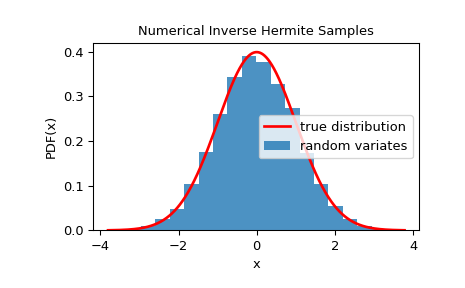
To check that the random variates closely follow the given distribution, we can look at its histogram:
>>> dist = StandardNormal()
>>> urng = np.random.default_rng()
>>> rng = NumericalInverseHermite(dist, random_state=urng)
>>> rvs = rng.rvs(10000)
>>> x = np.linspace(rvs.min()-0.1, rvs.max()+0.1, 1000)
>>> fx = norm.pdf(x)
>>> plt.plot(x, fx, 'r-', lw=2, label='true distribution')
>>> plt.hist(rvs, bins=20, density=True, alpha=0.8, label='random variates')
>>> plt.xlabel('x')
>>> plt.ylabel('PDF(x)')
>>> plt.title('Numerical Inverse Hermite Samples')
>>> plt.legend()
>>> plt.show()
Given the derivative of the PDF w.r.t the variate (i.e. x), we can use
quintic Hermite interpolation to approximate the PPF by passing the order
parameter:
>>> class StandardNormal:
...     def pdf(self, x):
...        return 1/np.sqrt(2*np.pi) * np.exp(-x**2 / 2)
...     def dpdf(self, x):
...        return -1/np.sqrt(2*np.pi) * x * np.exp(-x**2 / 2)
...     def cdf(self, x):
...        return ndtr(x)
...
>>> dist = StandardNormal()
>>> urng = np.random.default_rng()
>>> rng = NumericalInverseHermite(dist, order=5, random_state=urng)
Higher orders result in a fewer number of intervals:
>>> rng3 = NumericalInverseHermite(dist, order=3)
>>> rng5 = NumericalInverseHermite(dist, order=5)
>>> rng3.intervals, rng5.intervals
(3000, 522)
The u-error can be estimated by calling the u_error method. It runs a small Monte-Carlo simulation to estimate the u-error. By default, 100,000 samples are used. This can be changed by passing the sample_size argument:
>>> rng1 = NumericalInverseHermite(dist, u_resolution=1e-10)
>>> rng1.u_error(sample_size=1000000)  # uses one million samples
UError(max_error=9.53167544892608e-11, mean_absolute_error=2.2450136432146864e-11)
This returns a namedtuple which contains the maximum u-error and the mean absolute u-error.
The u-error can be reduced by decreasing the u-resolution (maximum allowed u-error):
>>> rng2 = NumericalInverseHermite(dist, u_resolution=1e-13)
>>> rng2.u_error(sample_size=1000000)
UError(max_error=9.32027892364129e-14, mean_absolute_error=1.5194172675685075e-14)
Note that this comes at the cost of computation time as a result of the increased setup time and number of intervals.
>>> rng1.intervals
1022
>>> rng2.intervals
5687
>>> from timeit import timeit
>>> f = lambda: NumericalInverseHermite(dist, u_resolution=1e-10)
>>> timeit(f, number=1)
0.017409582000254886  # may vary
>>> f = lambda: NumericalInverseHermite(dist, u_resolution=1e-13)
>>> timeit(f, number=1)
0.08671202100003939  # may vary
See 1 and 2 for more details on this method.
References#
- 1(1,2)
Hörmann, Wolfgang, and Josef Leydold. “Continuous random variate generation by fast numerical inversion.” ACM Transactions on Modeling and Computer Simulation (TOMACS) 13.4 (2003): 347-362.
- 2
UNU.RAN reference manual, Section 5.3.5, “HINV - Hermite interpolation based INVersion of CDF”, https://statmath.wu.ac.at/software/unuran/doc/unuran.html#HINV