scipy.stats.sampling.NumericalInverseHermite#

class scipy.stats.sampling.NumericalInverseHermite(dist, *, domain=None, order=3, u_resolution=1e-12, construction_points=None, random_state=None)#

Hermite interpolation based INVersion of CDF (HINV).

HINV is a variant of numerical inversion, where the inverse CDF is approximated using Hermite interpolation, i.e., the interval [0,1] is split into several intervals and in each interval the inverse CDF is approximated by polynomials constructed by means of values of the CDF and PDF at interval boundaries. This makes it possible to improve the accuracy by splitting a particular interval without recomputations in unaffected intervals. Three types of splines are implemented: linear, cubic, and quintic interpolation. For linear interpolation only the CDF is required. Cubic interpolation also requires PDF and quintic interpolation PDF and its derivative.

These splines have to be computed in a setup step. However, it only works for distributions with bounded domain; for distributions with unbounded domain the tails are chopped off such that the probability for the tail regions is small compared to the given u-resolution.

The method is not exact, as it only produces random variates of the approximated distribution. Nevertheless, the maximal numerical error in “u-direction” (i.e. |U - CDF(X)| where X is the approximate percentile corresponding to the quantile U i.e. X = approx_ppf(U)) can be set to the required resolution (within machine precision). Notice that very small values of the u-resolution are possible but may increase the cost for the setup step.

Parameters

distobject

An instance of a class with a cdf and optionally a pdf and dpdf method.

cdf: CDF of the distribution. The signature of the CDF is expected to be: def cdf(self, x: float) -> float. i.e. the CDF should accept a Python float and return a Python float.
pdf: PDF of the distribution. This method is optional when order=1. Must have the same signature as the PDF.
dpdf: Derivative of the PDF w.r.t the variate (i.e. x). This method is optional with order=1 or order=3. Must have the same signature as the CDF.

domainlist or tuple of length 2, optional

The support of the distribution. Default is None. When None:

If a support method is provided by the distribution object dist, it is used to set the domain of the distribution.
Otherwise the support is assumed to be \((-\infty, \infty)\).

orderint, default: 3

Set order of Hermite interpolation. Valid orders are 1, 3, and 5. Valid orders are 1, 3, and 5. Notice that order greater than 1 requires the density of the distribution, and order greater than 3 even requires the derivative of the density. Using order 1 results for most distributions in a huge number of intervals and is therefore not recommended. If the maximal error in u-direction is very small (say smaller than 1.e-10), order 5 is recommended as it leads to considerably fewer design points, as long there are no poles or heavy tails.

u_resolutionfloat, default: 1e-12

Set maximal tolerated u-error. Notice that the resolution of most uniform random number sources is 2-32= 2.3e-10. Thus a value of 1.e-10 leads to an inversion algorithm that could be called exact. For most simulations slightly bigger values for the maximal error are enough as well. Default is 1e-12.

construction_pointsarray_like, optional

Set starting construction points (nodes) for Hermite interpolation. As the possible maximal error is only estimated in the setup it may be necessary to set some special design points for computing the Hermite interpolation to guarantee that the maximal u-error can not be bigger than desired. Such points are points where the density is not differentiable or has a local extremum.

random_state{None, int, numpy.random.Generator,

numpy.random.RandomState}, optional

A NumPy random number generator or seed for the underlying NumPy random number generator used to generate the stream of uniform random numbers. If random_state is None (or np.random), the numpy.random.RandomState singleton is used. If random_state is an int, a new RandomState instance is used, seeded with random_state. If random_state is already a Generator or RandomState instance then that instance is used.

Notes

NumericalInverseHermite approximates the inverse of a continuous statistical distribution’s CDF with a Hermite spline. Order of the hermite spline can be specified by passing the order parameter.

As described in [1], it begins by evaluating the distribution’s PDF and CDF at a mesh of quantiles x within the distribution’s support. It uses the results to fit a Hermite spline H such that H(p) == x, where p is the array of percentiles corresponding with the quantiles x. Therefore, the spline approximates the inverse of the distribution’s CDF to machine precision at the percentiles p, but typically, the spline will not be as accurate at the midpoints between the percentile points:

p_mid = (p[:-1] + p[1:])/2

so the mesh of quantiles is refined as needed to reduce the maximum “u-error”:

u_error = np.max(np.abs(dist.cdf(H(p_mid)) - p_mid))

below the specified tolerance u_resolution. Refinement stops when the required tolerance is achieved or when the number of mesh intervals after the next refinement could exceed the maximum allowed number of intervals, which is 100000.

This method accepted a tol parameter to specify the maximum tolerable u-error but it has now been deprecated in the favor of u_resolution. tol will be removed completely in a future release.

References

1: Hörmann, Wolfgang, and Josef Leydold. “Continuous random variate generation by fast numerical inversion.” ACM Transactions on Modeling and Computer Simulation (TOMACS) 13.4 (2003): 347-362.
2: UNU.RAN reference manual, Section 5.3.5, “HINV - Hermite interpolation based INVersion of CDF”, https://statmath.wu.ac.at/software/unuran/doc/unuran.html#HINV

Examples

>>> from scipy.stats.sampling import NumericalInverseHermite
>>> from scipy.stats import norm, genexpon
>>> from scipy.special import ndtr

To create a generator to sample from the standard normal distribution, do:

>>> class StandardNormal:
...     def pdf(self, x):
...        return 1/np.sqrt(2*np.pi) * np.exp(-x**2 / 2)
...     def cdf(self, x):
...        return ndtr(x)
... 
>>> dist = StandardNormal()
>>> urng = np.random.default_rng()
>>> rng = NumericalInverseHermite(dist, random_state=urng)

The NumericalInverseHermite has a method that approximates the PPF of the distribution.

>>> rng = NumericalInverseHermite(dist)
>>> p = np.linspace(0.01, 0.99, 99) # percentiles from 1% to 99%
>>> np.allclose(rng.ppf(p), norm.ppf(p))
True

Depending on the implementation of the distribution’s random sampling method, the random variates generated may be nearly identical, given the same random state.

>>> dist = genexpon(9, 16, 3)
>>> rng = NumericalInverseHermite(dist)
>>> # `seed` ensures identical random streams are used by each `rvs` method
>>> seed = 500072020
>>> rvs1 = dist.rvs(size=100, random_state=np.random.default_rng(seed))
>>> rvs2 = rng.rvs(size=100, random_state=np.random.default_rng(seed))
>>> np.allclose(rvs1, rvs2)
True

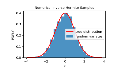
To check that the random variates closely follow the given distribution, we can look at its histogram:

>>> import matplotlib.pyplot as plt
>>> dist = StandardNormal()
>>> rng = NumericalInverseHermite(dist)
>>> rvs = rng.rvs(10000)
>>> x = np.linspace(rvs.min()-0.1, rvs.max()+0.1, 1000)
>>> fx = norm.pdf(x)
>>> plt.plot(x, fx, 'r-', lw=2, label='true distribution')
>>> plt.hist(rvs, bins=20, density=True, alpha=0.8, label='random variates')
>>> plt.xlabel('x')
>>> plt.ylabel('PDF(x)')
>>> plt.title('Numerical Inverse Hermite Samples')
>>> plt.legend()
>>> plt.show()

../../_images/scipy-stats-sampling-NumericalInverseHermite-1_00_00.png

Given the derivative of the PDF w.r.t the variate (i.e. x), we can use quintic Hermite interpolation to approximate the PPF by passing the order parameter:

>>> class StandardNormal:
...     def pdf(self, x):
...        return 1/np.sqrt(2*np.pi) * np.exp(-x**2 / 2)
...     def dpdf(self, x):
...        return -1/np.sqrt(2*np.pi) * x * np.exp(-x**2 / 2)
...     def cdf(self, x):
...        return ndtr(x)
... 
>>> dist = StandardNormal()
>>> urng = np.random.default_rng()
>>> rng = NumericalInverseHermite(dist, order=5, random_state=urng)

Higher orders result in a fewer number of intervals:

>>> rng3 = NumericalInverseHermite(dist, order=3)
>>> rng5 = NumericalInverseHermite(dist, order=5)
>>> rng3.intervals, rng5.intervals
(3000, 522)

The u-error can be estimated by calling the u_error method. It runs a small Monte-Carlo simulation to estimate the u-error. By default, 100,000 samples are used. This can be changed by passing the sample_size argument:

>>> rng1 = NumericalInverseHermite(dist, u_resolution=1e-10)
>>> rng1.u_error(sample_size=1000000)  # uses one million samples
UError(max_error=9.53167544892608e-11, mean_absolute_error=2.2450136432146864e-11)

This returns a namedtuple which contains the maximum u-error and the mean absolute u-error.

The u-error can be reduced by decreasing the u-resolution (maximum allowed u-error):

>>> rng2 = NumericalInverseHermite(dist, u_resolution=1e-13)
>>> rng2.u_error(sample_size=1000000)
UError(max_error=9.32027892364129e-14, mean_absolute_error=1.5194172675685075e-14)

Note that this comes at the cost of increased setup time and number of intervals.

>>> rng1.intervals
1022
>>> rng2.intervals
5687
>>> from timeit import timeit
>>> f = lambda: NumericalInverseHermite(dist, u_resolution=1e-10)
>>> timeit(f, number=1)
0.017409582000254886  # may vary
>>> f = lambda: NumericalInverseHermite(dist, u_resolution=1e-13)
>>> timeit(f, number=1)
0.08671202100003939  # may vary

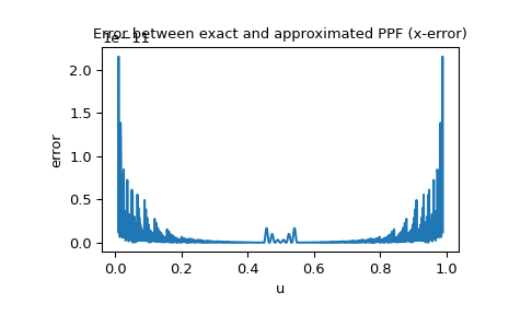
Since the PPF of the normal distribution is available as a special function, we can also check the x-error, i.e. the difference between the approximated PPF and exact PPF:

>>> import matplotlib.pyplot as plt
>>> u = np.linspace(0.01, 0.99, 1000)
>>> approxppf = rng.ppf(u)
>>> exactppf = norm.ppf(u)
>>> error = np.abs(exactppf - approxppf)
>>> plt.plot(u, error)
>>> plt.xlabel('u')
>>> plt.ylabel('error')
>>> plt.title('Error between exact and approximated PPF (x-error)')
>>> plt.show()

../../_images/scipy-stats-sampling-NumericalInverseHermite-1_01_00.png

Attributes

intervals: Get number of nodes (design points) used for Hermite interpolation in the generator object.
midpoint_error

Methods

`ppf`(u)	Approximated PPF of the given distribution.
`qrvs`([size, d, qmc_engine])	Quasi-random variates of the given RV.
`rvs`([size, random_state])	Sample from the distribution.
`set_random_state`([random_state])	Set the underlying uniform random number generator.
`u_error`([sample_size])	Estimate the u-error of the approximation using Monte Carlo simulation.

Random Number Generators (scipy.stats.sampling)

scipy.stats.sampling.NumericalInverseHermite.ppf