scipy.special.nbdtrc#

scipy.special.nbdtrc(k, n, p, out=None) = <ufunc 'nbdtrc'>#

Negative binomial survival function.

Returns the sum of the terms k + 1 to infinity of the negative binomial distribution probability mass function,

\[F = \sum_{j=k + 1}^\infty {{n + j - 1}\choose{j}} p^n (1 - p)^j.\]

In a sequence of Bernoulli trials with individual success probabilities p, this is the probability that more than k failures precede the nth success.

Parameters:

karray_like: The maximum number of allowed failures (nonnegative int).
narray_like: The target number of successes (positive int).
parray_like: Probability of success in a single event (float).
outndarray, optional: Optional output array for the function results

Returns:

Fscalar or ndarray: The probability of k + 1 or more failures before n successes in a sequence of events with individual success probability p.

See also

nbdtr: Negative binomial cumulative distribution function
nbdtrik: Negative binomial percentile function
scipy.stats.nbinom: Negative binomial distribution

Notes

If floating point values are passed for k or n, they will be truncated to integers.

The terms are not summed directly; instead the regularized incomplete beta function is employed, according to the formula,

\[\mathrm{nbdtrc}(k, n, p) = I_{1 - p}(k + 1, n).\]

Wrapper for the Cephes [1] routine nbdtrc.

The negative binomial distribution is also available as scipy.stats.nbinom. Using nbdtrc directly can improve performance compared to the sf method of scipy.stats.nbinom (see last example).

References

[1]

Cephes Mathematical Functions Library, http://www.netlib.org/cephes/

Examples

Compute the function for k=10 and n=5 at p=0.5.

>>> import numpy as np
>>> from scipy.special import nbdtrc
>>> nbdtrc(10, 5, 0.5)
0.059234619140624986

Compute the function for n=10 and p=0.5 at several points by providing a NumPy array or list for k.

>>> nbdtrc([5, 10, 15], 10, 0.5)
array([0.84912109, 0.41190147, 0.11476147])

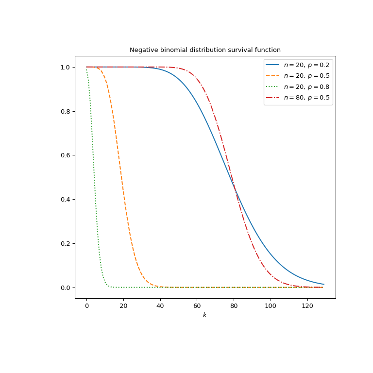
Plot the function for four different parameter sets.

>>> import matplotlib.pyplot as plt
>>> k = np.arange(130)
>>> n_parameters = [20, 20, 20, 80]
>>> p_parameters = [0.2, 0.5, 0.8, 0.5]
>>> linestyles = ['solid', 'dashed', 'dotted', 'dashdot']
>>> parameters_list = list(zip(p_parameters, n_parameters,
...                            linestyles))
>>> fig, ax = plt.subplots(figsize=(8, 8))
>>> for parameter_set in parameters_list:
...     p, n, style = parameter_set
...     nbdtrc_vals = nbdtrc(k, n, p)
...     ax.plot(k, nbdtrc_vals, label=rf"$n={n},\, p={p}$",
...             ls=style)
>>> ax.legend()
>>> ax.set_xlabel("$k$")
>>> ax.set_title("Negative binomial distribution survival function")
>>> plt.show()

../../_images/scipy-special-nbdtrc-1_00_00.png

The negative binomial distribution is also available as scipy.stats.nbinom. Using nbdtrc directly can be much faster than calling the sf method of scipy.stats.nbinom, especially for small arrays or individual values. To get the same results one must use the following parametrization: nbinom(n, p).sf(k)=nbdtrc(k, n, p).

>>> from scipy.stats import nbinom
>>> k, n, p = 3, 5, 0.5
>>> nbdtr_res = nbdtrc(k, n, p)  # this will often be faster than below
>>> stats_res = nbinom(n, p).sf(k)
>>> stats_res, nbdtr_res  # test that results are equal
(0.6367187499999999, 0.6367187499999999)

nbdtrc can evaluate different parameter sets by providing arrays with shapes compatible for broadcasting for k, n and p. Here we compute the function for three different k at four locations p, resulting in a 3x4 array.

>>> k = np.array([[5], [10], [15]])
>>> p = np.array([0.3, 0.5, 0.7, 0.9])
>>> k.shape, p.shape
((3, 1), (4,))

>>> nbdtrc(k, 5, p)
array([[8.49731667e-01, 3.76953125e-01, 4.73489874e-02, 1.46902600e-04],
       [5.15491059e-01, 5.92346191e-02, 6.72234070e-04, 9.29610100e-09],
       [2.37507779e-01, 5.90896606e-03, 5.55025308e-06, 3.26346760e-13]])