scipy.special.gamma#

scipy.special.gamma(z, out=None) = <ufunc 'gamma'>#

gamma function.

The gamma function is defined as

\[\Gamma(z) = \int_0^\infty t^{z-1} e^{-t} dt\]

for \(\Re(z) > 0\) and is extended to the rest of the complex plane by analytic continuation. See [dlmf] for more details.

Parameters:

zarray_like: Real or complex valued argument
outndarray, optional: Optional output array for the function values

Returns:

scalar or ndarray: Values of the gamma function

Notes

The gamma function is often referred to as the generalized factorial since \(\Gamma(n + 1) = n!\) for natural numbers \(n\). More generally it satisfies the recurrence relation \(\Gamma(z + 1) = z \cdot \Gamma(z)\) for complex \(z\), which, combined with the fact that \(\Gamma(1) = 1\), implies the above identity for \(z = n\).

References

[dlmf]

NIST Digital Library of Mathematical Functions https://dlmf.nist.gov/5.2#E1

Examples

>>> import numpy as np
>>> from scipy.special import gamma, factorial

>>> gamma([0, 0.5, 1, 5])
array([         inf,   1.77245385,   1.        ,  24.        ])

>>> z = 2.5 + 1j
>>> gamma(z)
(0.77476210455108352+0.70763120437959293j)
>>> gamma(z+1), z*gamma(z)  # Recurrence property
((1.2292740569981171+2.5438401155000685j),
 (1.2292740569981158+2.5438401155000658j))

>>> gamma(0.5)**2  # gamma(0.5) = sqrt(pi)
3.1415926535897927

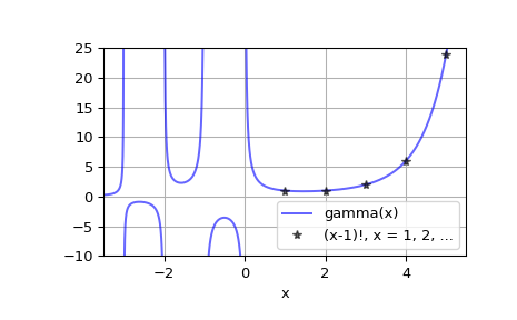
Plot gamma(x) for real x

>>> x = np.linspace(-3.5, 5.5, 2251)
>>> y = gamma(x)

>>> import matplotlib.pyplot as plt
>>> plt.plot(x, y, 'b', alpha=0.6, label='gamma(x)')
>>> k = np.arange(1, 7)
>>> plt.plot(k, factorial(k-1), 'k*', alpha=0.6,
...          label='(x-1)!, x = 1, 2, ...')
>>> plt.xlim(-3.5, 5.5)
>>> plt.ylim(-10, 25)
>>> plt.grid()
>>> plt.xlabel('x')
>>> plt.legend(loc='lower right')
>>> plt.show()