scipy.special.gamma

scipy.special.gamma(z, out=None) = <ufunc 'gamma'>

gamma function.

The gamma function is defined as

\[\Gamma(z) = \int_0^\infty t^{z-1} e^{-t} dt\]

for \(\Re(z) > 0\) and is extended to the rest of the complex plane by analytic continuation. See [dlmf] for more details.

Parameters

zarray_like

Real or complex valued argument

outndarray, optional

Optional output array for the function values

Returns

scalar or ndarray

Values of the gamma function

Notes

The gamma function is often referred to as the generalized factorial since \(\Gamma(n + 1) = n!\) for natural numbers \(n\). More generally it satisfies the recurrence relation \(\Gamma(z + 1) = z \cdot \Gamma(z)\) for complex \(z\), which, combined with the fact that \(\Gamma(1) = 1\), implies the above identity for \(z = n\).

References

dlmf

NIST Digital Library of Mathematical Functions https://dlmf.nist.gov/5.2#E1

Examples

>>> from scipy.special import gamma, factorial

>>> gamma([0, 0.5, 1, 5])
array([         inf,   1.77245385,   1.        ,  24.        ])

>>> z = 2.5 + 1j
>>> gamma(z)
(0.77476210455108352+0.70763120437959293j)
>>> gamma(z+1), z*gamma(z)  # Recurrence property
((1.2292740569981171+2.5438401155000685j),
 (1.2292740569981158+2.5438401155000658j))

>>> gamma(0.5)**2  # gamma(0.5) = sqrt(pi)
3.1415926535897927

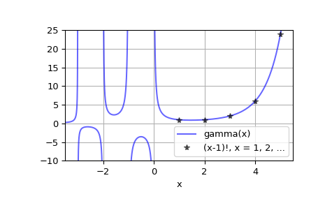
Plot gamma(x) for real x

>>> x = np.linspace(-3.5, 5.5, 2251)
>>> y = gamma(x)

>>> import matplotlib.pyplot as plt
>>> plt.plot(x, y, 'b', alpha=0.6, label='gamma(x)')
>>> k = np.arange(1, 7)
>>> plt.plot(k, factorial(k-1), 'k*', alpha=0.6,
...          label='(x-1)!, x = 1, 2, ...')
>>> plt.xlim(-3.5, 5.5)
>>> plt.ylim(-10, 25)
>>> plt.grid()
>>> plt.xlabel('x')
>>> plt.legend(loc='lower right')
>>> plt.show()