geometric_slerp#
- scipy.spatial.geometric_slerp(start, end, t, tol=1e-07)[source]#
Geometric spherical linear interpolation.
The interpolation occurs along a unit-radius great circle arc in arbitrary dimensional space.
- Parameters:
- start(n_dimensions, ) array-like
Single n-dimensional input coordinate in a 1-D array-like object. n must be greater than 1.
- end(n_dimensions, ) array-like
Single n-dimensional input coordinate in a 1-D array-like object. n must be greater than 1.
- tfloat or (n_points,) 1D array-like
A float or 1D array-like of doubles representing interpolation parameters. A common approach is to generate the array with
np.linspace(0, 1, n_pts)for linearly spaced points. Ascending, descending, and scrambled orders are permitted.Changed in version 1.17.0: Extrapolation is permitted, allowing values below 0 and above 1.
- tolfloat
The absolute tolerance for determining if the start and end coordinates are antipodes.
- Returns:
- result(t.size, D)
An array of doubles containing the interpolated spherical path and including start and end when 0 and 1 t are used. The interpolated values should correspond to the same sort order provided in the t array. The result may be 1-dimensional if
tis a float.
- Raises:
- ValueError
If
startorendare not on the unit n-sphere, or for a variety of degenerate conditions.
See also
scipy.spatial.transform.Slerp3-D Slerp that works with quaternions
Notes
The implementation is based on the mathematical formula provided in [1], and the first known presentation of this algorithm, derived from study of 4-D geometry, is credited to Glenn Davis in a footnote of the original quaternion Slerp publication by Ken Shoemake [2].
Added in version 1.5.0.
References
[2]Ken Shoemake (1985) Animating rotation with quaternion curves. ACM SIGGRAPH Computer Graphics, 19(3): 245-254.
Examples
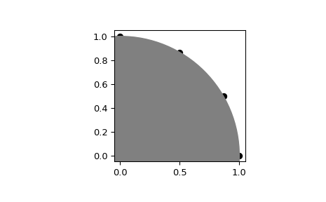
Interpolate four linearly-spaced values on the circumference of a circle spanning 90 degrees:
>>> import numpy as np
>>> from scipy.spatial import geometric_slerp
>>> import matplotlib.pyplot as plt
>>> fig = plt.figure()
>>> ax = fig.add_subplot(111)
>>> start = np.array([1, 0])
>>> end = np.array([0, 1])
>>> t_vals = np.linspace(0, 1, 4)
>>> result = geometric_slerp(start,
...                          end,
...                          t_vals)
The interpolated results should be at 30 degree intervals recognizable on the unit circle:
>>> ax.scatter(result[...,0], result[...,1], c='k')
>>> circle = plt.Circle((0, 0), 1, color='grey')
>>> ax.add_artist(circle)
>>> ax.set_aspect('equal')
>>> plt.show()
Attempting to interpolate between antipodes on a circle is ambiguous because there are two possible paths, and on a sphere there are infinite possible paths on the geodesic surface. Nonetheless, one of the ambiguous paths is returned along with a warning:
>>> import warnings
>>> opposite_pole = np.array([-1, 0])
>>> with warnings.catch_warnings():
...     warnings.simplefilter("ignore", UserWarning)
...     geometric_slerp(start,
...                     opposite_pole,
...                     t_vals)
array([[ 1.00000000e+00,  0.00000000e+00],
       [ 5.00000000e-01,  8.66025404e-01],
       [-5.00000000e-01,  8.66025404e-01],
       [-1.00000000e+00,  1.22464680e-16]])
Extend the original example to a sphere and plot interpolation points in 3D:
>>> from mpl_toolkits.mplot3d import proj3d
>>> fig = plt.figure()
>>> ax = fig.add_subplot(111, projection='3d')
Plot the unit sphere for reference (optional):
>>> u = np.linspace(0, 2 * np.pi, 100)
>>> v = np.linspace(0, np.pi, 100)
>>> x = np.outer(np.cos(u), np.sin(v))
>>> y = np.outer(np.sin(u), np.sin(v))
>>> z = np.outer(np.ones(np.size(u)), np.cos(v))
>>> ax.plot_surface(x, y, z, color='y', alpha=0.1)
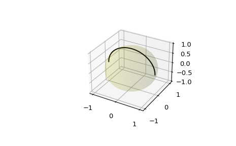
Interpolating over a larger number of points may provide the appearance of a smooth curve on the surface of the sphere, which is also useful for discretized integration calculations on a sphere surface:
>>> start = np.array([1, 0, 0])
>>> end = np.array([0, 0, 1])
>>> t_vals = np.linspace(0, 1, 200)
>>> result = geometric_slerp(start,
...                          end,
...                          t_vals)
>>> ax.plot(result[...,0],
...         result[...,1],
...         result[...,2],
...         c='k')
>>> plt.show()
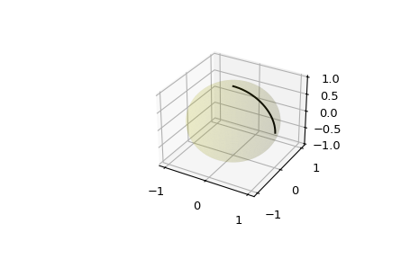
It is also possible to perform extrapolations outside the interpolation interval by using interpolation parameter values below 0 or above 1. For example, the above example may be adjusted to extrapolate to an antipodal position:
>>> fig = plt.figure()
>>> ax = fig.add_subplot(111, projection='3d')
>>> ax.plot_surface(x, y, z, color='y', alpha=0.1)
>>> start = np.array([1, 0, 0])
>>> end = np.array([0, 0, 1])
>>> t_vals = np.linspace(0, 2, 400)
>>> result = geometric_slerp(start,
...                          end,
...                          t_vals)
>>> ax.plot(result[...,0], result[...,1], result[...,2], c='k')
>>> plt.show()