scipy.signal.iircomb

scipy.signal.iircomb(w0, Q, ftype='notch', fs=2.0, *, pass_zero=False)

Design IIR notching or peaking digital comb filter.

A notching comb filter consists of regularly-spaced band-stop filters with a narrow bandwidth (high quality factor). Each rejects a narrow frequency band and leaves the rest of the spectrum little changed.

A peaking comb filter consists of regularly-spaced band-pass filters with a narrow bandwidth (high quality factor). Each rejects components outside a narrow frequency band.

Parameters:

w0float

The fundamental frequency of the comb filter (the spacing between its peaks). This must evenly divide the sampling frequency. If fs is specified, this is in the same units as fs. By default, it is a normalized scalar that must satisfy 0 < w0 < 1, with w0 = 1 corresponding to half of the sampling frequency.

Qfloat

Quality factor. Dimensionless parameter that characterizes notch filter -3 dB bandwidth bw relative to its center frequency, Q = w0/bw.

ftype{‘notch’, ‘peak’}

The type of comb filter generated by the function. If ‘notch’, then the Q factor applies to the notches. If ‘peak’, then the Q factor applies to the peaks. Default is ‘notch’.

fsfloat, optional

The sampling frequency of the signal. Default is 2.0.

pass_zerobool, optional

If False (default), the notches (nulls) of the filter are centered on frequencies [0, w0, 2*w0, …], and the peaks are centered on the midpoints [w0/2, 3*w0/2, 5*w0/2, …]. If True, the peaks are centered on [0, w0, 2*w0, …] (passing zero frequency) and vice versa.

New in version 1.9.0.

Returns:

b, andarray, ndarray

Numerator (b) and denominator (a) polynomials of the IIR filter.

Raises:

ValueError

If w0 is less than or equal to 0 or greater than or equal to fs/2, if fs is not divisible by w0, if ftype is not ‘notch’ or ‘peak’

See also

iirnotch

iirpeak

Notes

For implementation details, see [1]. The TF implementation of the comb filter is numerically stable even at higher orders due to the use of a single repeated pole, which won’t suffer from precision loss.

References

[1]

Sophocles J. Orfanidis, “Introduction To Signal Processing”, Prentice-Hall, 1996, ch. 11, “Digital Filter Design”

Examples

Try it in your browser!

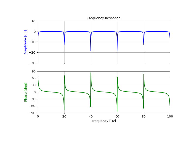
Design and plot notching comb filter at 20 Hz for a signal sampled at 200 Hz, using quality factor Q = 30

>>> from scipy import signal
>>> import matplotlib.pyplot as plt
>>> import numpy as np

>>> fs = 200.0  # Sample frequency (Hz)
>>> f0 = 20.0  # Frequency to be removed from signal (Hz)
>>> Q = 30.0  # Quality factor
>>> # Design notching comb filter
>>> b, a = signal.iircomb(f0, Q, ftype='notch', fs=fs)

>>> # Frequency response
>>> freq, h = signal.freqz(b, a, fs=fs)
>>> response = abs(h)
>>> # To avoid divide by zero when graphing
>>> response[response == 0] = 1e-20
>>> # Plot
>>> fig, ax = plt.subplots(2, 1, figsize=(8, 6), sharex=True)
>>> ax[0].plot(freq, 20*np.log10(abs(response)), color='blue')
>>> ax[0].set_title("Frequency Response")
>>> ax[0].set_ylabel("Amplitude (dB)", color='blue')
>>> ax[0].set_xlim([0, 100])
>>> ax[0].set_ylim([-30, 10])
>>> ax[0].grid(True)
>>> ax[1].plot(freq, (np.angle(h)*180/np.pi+180)%360 - 180, color='green')
>>> ax[1].set_ylabel("Angle (degrees)", color='green')
>>> ax[1].set_xlabel("Frequency (Hz)")
>>> ax[1].set_xlim([0, 100])
>>> ax[1].set_yticks([-90, -60, -30, 0, 30, 60, 90])
>>> ax[1].set_ylim([-90, 90])
>>> ax[1].grid(True)
>>> plt.show()

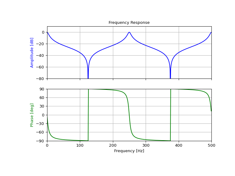
Design and plot peaking comb filter at 250 Hz for a signal sampled at 1000 Hz, using quality factor Q = 30

>>> fs = 1000.0  # Sample frequency (Hz)
>>> f0 = 250.0  # Frequency to be retained (Hz)
>>> Q = 30.0  # Quality factor
>>> # Design peaking filter
>>> b, a = signal.iircomb(f0, Q, ftype='peak', fs=fs, pass_zero=True)

>>> # Frequency response
>>> freq, h = signal.freqz(b, a, fs=fs)
>>> response = abs(h)
>>> # To avoid divide by zero when graphing
>>> response[response == 0] = 1e-20
>>> # Plot
>>> fig, ax = plt.subplots(2, 1, figsize=(8, 6), sharex=True)
>>> ax[0].plot(freq, 20*np.log10(np.maximum(abs(h), 1e-5)), color='blue')
>>> ax[0].set_title("Frequency Response")
>>> ax[0].set_ylabel("Amplitude (dB)", color='blue')
>>> ax[0].set_xlim([0, 500])
>>> ax[0].set_ylim([-80, 10])
>>> ax[0].grid(True)
>>> ax[1].plot(freq, (np.angle(h)*180/np.pi+180)%360 - 180, color='green')
>>> ax[1].set_ylabel("Angle (degrees)", color='green')
>>> ax[1].set_xlabel("Frequency (Hz)")
>>> ax[1].set_xlim([0, 500])
>>> ax[1].set_yticks([-90, -60, -30, 0, 30, 60, 90])
>>> ax[1].set_ylim([-90, 90])
>>> ax[1].grid(True)
>>> plt.show()

Go BackOpen In Tab