scipy.interpolate.

splrep

scipy.interpolate.splrep(x, y, w=None, xb=None, xe=None, k=3, task=0, s=None, t=None, full_output=0, per=0, quiet=1)

Find the B-spline representation of a 1-D curve.

Given the set of data points (x[i], y[i]) determine a smooth spline approximation of degree k on the interval xb <= x <= xe.

Parameters:

x, yarray_like

The data points defining a curve y = f(x).

warray_like, optional

Strictly positive rank-1 array of weights the same length as x and y. The weights are used in computing the weighted least-squares spline fit. If the errors in the y values have standard-deviation given by the vector d, then w should be 1/d. Default is ones(len(x)).

xb, xefloat, optional

The interval to fit. If None, these default to x[0] and x[-1] respectively.

kint, optional

The degree of the spline fit. It is recommended to use cubic splines. Even values of k should be avoided especially with small s values. 1 <= k <= 5.

task{1, 0, -1}, optional

If task==0, find t and c for a given smoothing factor, s.

If task==1 find t and c for another value of the smoothing factor, s. There must have been a previous call with task=0 or task=1 for the same set of data (t will be stored an used internally)

If task=-1 find the weighted least square spline for a given set of knots, t. These should be interior knots as knots on the ends will be added automatically.

sfloat, optional

A smoothing condition. The amount of smoothness is determined by satisfying the conditions: sum((w * (y - g))**2,axis=0) <= s where g(x) is the smoothed interpolation of (x,y). The user can use s to control the tradeoff between closeness and smoothness of fit. Larger s means more smoothing while smaller values of s indicate less smoothing. Recommended values of s depend on the weights, w. If the weights represent the inverse of the standard-deviation of y, then a good s value should be found in the range (m-sqrt(2*m),m+sqrt(2*m)) where m is the number of datapoints in x, y, and w. default : s=m-sqrt(2*m) if weights are supplied. s = 0.0 (interpolating) if no weights are supplied.

tarray_like, optional

The knots needed for task=-1. If given then task is automatically set to -1.

full_outputbool, optional

If non-zero, then return optional outputs.

perbool, optional

If non-zero, data points are considered periodic with period x[m-1] - x[0] and a smooth periodic spline approximation is returned. Values of y[m-1] and w[m-1] are not used. The default is zero, corresponding to boundary condition ‘not-a-knot’.

quietbool, optional

Non-zero to suppress messages.

Returns:

tcktuple

A tuple (t,c,k) containing the vector of knots, the B-spline coefficients, and the degree of the spline.

fparray, optional

The weighted sum of squared residuals of the spline approximation.

ierint, optional

An integer flag about splrep success. Success is indicated if ier<=0. If ier in [1,2,3], an error occurred but was not raised. Otherwise an error is raised.

msgstr, optional

A message corresponding to the integer flag, ier.

See also

UnivariateSpline, BivariateSpline

splprep, splev, sproot, spalde, splint

bisplrep, bisplev

BSpline

make_interp_spline

Notes

See splev for evaluation of the spline and its derivatives. Uses the FORTRAN routine curfit from FITPACK.

The user is responsible for assuring that the values of x are unique. Otherwise, splrep will not return sensible results.

If provided, knots t must satisfy the Schoenberg-Whitney conditions, i.e., there must be a subset of data points x[j] such that t[j] < x[j] < t[j+k+1], for j=0, 1,...,n-k-2.

This routine zero-pads the coefficients array c to have the same length as the array of knots t (the trailing k + 1 coefficients are ignored by the evaluation routines, splev and BSpline.) This is in contrast with splprep, which does not zero-pad the coefficients.

The default boundary condition is ‘not-a-knot’, i.e. the first and second segment at a curve end are the same polynomial. More boundary conditions are available in CubicSpline.

References

Based on algorithms described in [1], [2], [3], and [4]:

[1]

P. Dierckx, “An algorithm for smoothing, differentiation and integration of experimental data using spline functions”, J.Comp.Appl.Maths 1 (1975) 165-184.

[2]

P. Dierckx, “A fast algorithm for smoothing data on a rectangular grid while using spline functions”, SIAM J.Numer.Anal. 19 (1982) 1286-1304.

[3]

P. Dierckx, “An improved algorithm for curve fitting with spline functions”, report tw54, Dept. Computer Science,K.U. Leuven, 1981.

[4]

P. Dierckx, “Curve and surface fitting with splines”, Monographs on Numerical Analysis, Oxford University Press, 1993.

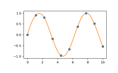
Examples

Try it in your browser!

You can interpolate 1-D points with a B-spline curve. Further examples are given in in the tutorial.

>>> import numpy as np
>>> import matplotlib.pyplot as plt
>>> from scipy.interpolate import splev, splrep
>>> x = np.linspace(0, 10, 10)
>>> y = np.sin(x)
>>> spl = splrep(x, y)
>>> x2 = np.linspace(0, 10, 200)
>>> y2 = splev(x2, spl)
>>> plt.plot(x, y, 'o', x2, y2)
>>> plt.show()

Go BackOpen In Tab