scipy.interpolate.

griddata#

scipy.interpolate.griddata(points, values, xi, method='linear', fill_value=nan, rescale=False)[source]#

Interpolate unstructured D-D data.

Parameters:

points2-D ndarray of floats with shape (n, D), or length D tuple of 1-D ndarrays with shape (n,).

Data point coordinates.

valuesndarray of float or complex, shape (n,)

Data values.

xi2-D ndarray of floats with shape (m, D), or length D tuple of ndarrays broadcastable to the same shape.

Points at which to interpolate data.

method{‘linear’, ‘nearest’, ‘cubic’}, optional

Method of interpolation. One of

nearest: return the value at the data point closest to the point of interpolation. See NearestNDInterpolator for more details.
linear: tessellate the input point set to N-D simplices, and interpolate linearly on each simplex. See LinearNDInterpolator for more details.
cubic (1-D): return the value determined from a cubic spline.
cubic (2-D): return the value determined from a piecewise cubic, continuously differentiable (C1), and approximately curvature-minimizing polynomial surface. See CloughTocher2DInterpolator for more details.

fill_valuefloat, optional

Value used to fill in for requested points outside of the convex hull of the input points. If not provided, then the default is nan. This option has no effect for the ‘nearest’ method.

rescalebool, optional

Rescale points to unit cube before performing interpolation. This is useful if some of the input dimensions have incommensurable units and differ by many orders of magnitude.

Added in version 0.14.0.

Returns:

ndarray: Array of interpolated values.

See also

LinearNDInterpolator: Piecewise linear interpolator in N dimensions.
NearestNDInterpolator: Nearest-neighbor interpolator in N dimensions.
CloughTocher2DInterpolator: Piecewise cubic, C1 smooth, curvature-minimizing interpolator in 2D.
interpn: Interpolation on a regular grid or rectilinear grid.
RegularGridInterpolator: Interpolator on a regular or rectilinear grid in arbitrary dimensions (interpn wraps this class).

Notes

Added in version 0.9.

Note

For data on a regular grid use interpn instead.

Examples

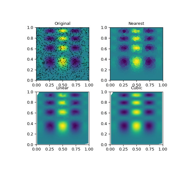
Suppose we want to interpolate the 2-D function

>>> import numpy as np
>>> def func(x, y):
...     return x*(1-x)*np.cos(4*np.pi*x) * np.sin(4*np.pi*y**2)**2

on a grid in [0, 1]x[0, 1]

>>> grid_x, grid_y = np.mgrid[0:1:100j, 0:1:200j]

but we only know its values at 1000 data points:

>>> rng = np.random.default_rng()
>>> points = rng.random((1000, 2))
>>> values = func(points[:,0], points[:,1])

This can be done with griddata – below we try out all of the interpolation methods:

>>> from scipy.interpolate import griddata
>>> grid_z0 = griddata(points, values, (grid_x, grid_y), method='nearest')
>>> grid_z1 = griddata(points, values, (grid_x, grid_y), method='linear')
>>> grid_z2 = griddata(points, values, (grid_x, grid_y), method='cubic')

One can see that the exact result is reproduced by all of the methods to some degree, but for this smooth function the piecewise cubic interpolant gives the best results:

>>> import matplotlib.pyplot as plt
>>> plt.subplot(221)
>>> plt.imshow(func(grid_x, grid_y).T, extent=(0,1,0,1), origin='lower')
>>> plt.plot(points[:,0], points[:,1], 'k.', ms=1)
>>> plt.title('Original')
>>> plt.subplot(222)
>>> plt.imshow(grid_z0.T, extent=(0,1,0,1), origin='lower')
>>> plt.title('Nearest')
>>> plt.subplot(223)
>>> plt.imshow(grid_z1.T, extent=(0,1,0,1), origin='lower')
>>> plt.title('Linear')
>>> plt.subplot(224)
>>> plt.imshow(grid_z2.T, extent=(0,1,0,1), origin='lower')
>>> plt.title('Cubic')
>>> plt.gcf().set_size_inches(6, 6)
>>> plt.show()

../../_images/scipy-interpolate-griddata-1.png