scipy.stats.irwinhall#
- scipy.stats.irwinhall = <scipy.stats._continuous_distns.irwinhall_gen object>[source]#
An Irwin-Hall (Uniform Sum) continuous random variable.
An Irwin-Hall continuous random variable is the sum of \(n\) independent standard uniform random variables [1] [2].
As an instance of the
rv_continuousclass,irwinhallobject inherits from it a collection of generic methods (see below for the full list), and completes them with details specific for this particular distribution.Methods
rvs(n, loc=0, scale=1, size=1, random_state=None)
Random variates.
pdf(x, n, loc=0, scale=1)
Probability density function.
logpdf(x, n, loc=0, scale=1)
Log of the probability density function.
cdf(x, n, loc=0, scale=1)
Cumulative distribution function.
logcdf(x, n, loc=0, scale=1)
Log of the cumulative distribution function.
sf(x, n, loc=0, scale=1)
Survival function (also defined as
1 - cdf, but sf is sometimes more accurate).logsf(x, n, loc=0, scale=1)
Log of the survival function.
ppf(q, n, loc=0, scale=1)
Percent point function (inverse of
cdf— percentiles).isf(q, n, loc=0, scale=1)
Inverse survival function (inverse of
sf).moment(order, n, loc=0, scale=1)
Non-central moment of the specified order.
stats(n, loc=0, scale=1, moments=’mv’)
Mean(‘m’), variance(‘v’), skew(‘s’), and/or kurtosis(‘k’).
entropy(n, loc=0, scale=1)
(Differential) entropy of the RV.
fit(data)
Parameter estimates for generic data. See scipy.stats.rv_continuous.fit for detailed documentation of the keyword arguments.
expect(func, args=(n,), loc=0, scale=1, lb=None, ub=None, conditional=False, **kwds)
Expected value of a function (of one argument) with respect to the distribution.
median(n, loc=0, scale=1)
Median of the distribution.
mean(n, loc=0, scale=1)
Mean of the distribution.
var(n, loc=0, scale=1)
Variance of the distribution.
std(n, loc=0, scale=1)
Standard deviation of the distribution.
interval(confidence, n, loc=0, scale=1)
Confidence interval with equal areas around the median.
Notes
Applications include Rao’s Spacing Test, a more powerful alternative to the Rayleigh test when the data are not unimodal, and radar [3].
Conveniently, the pdf and cdf are the \(n\)-fold convolution of the ones for the standard uniform distribution, which is also the definition of the cardinal B-splines of degree \(n-1\) having knots evenly spaced from \(1\) to \(n\) [4] [5].
The Bates distribution, which represents the mean of statistically independent, uniformly distributed random variables, is simply the Irwin-Hall distribution scaled by \(1/n\). For example, the frozen distribution
bates = irwinhall(10, scale=1/10)represents the distribution of the mean of 10 uniformly distributed random variables.The probability density above is defined in the “standardized” form. To shift and/or scale the distribution use the
locandscaleparameters. Specifically,irwinhall.pdf(x, n, loc, scale)is identically equivalent toirwinhall.pdf(y, n) / scalewithy = (x - loc) / scale. Note that shifting the location of a distribution does not make it a “noncentral” distribution; noncentral generalizations of some distributions are available in separate classes.References
[1]P. Hall, “The distribution of means for samples of size N drawn from a population in which the variate takes values between 0 and 1, all such values being equally probable”, Biometrika, Volume 19, Issue 3-4, December 1927, Pages 240-244, DOI:10.1093/biomet/19.3-4.240.
[2]J. O. Irwin, “On the frequency distribution of the means of samples from a population having any law of frequency with finite moments, with special reference to Pearson’s Type II, Biometrika, Volume 19, Issue 3-4, December 1927, Pages 225-239, DOI:0.1093/biomet/19.3-4.225.
[3]K. Buchanan, T. Adeyemi, C. Flores-Molina, S. Wheeland and D. Overturf, “Sidelobe behavior and bandwidth characteristics of distributed antenna arrays,” 2018 United States National Committee of URSI National Radio Science Meeting (USNC-URSI NRSM), Boulder, CO, USA, 2018, pp. 1-2. https://www.usnc-ursi-archive.org/nrsm/2018/papers/B15-9.pdf.
[4]Amos Ron, “Lecture 1: Cardinal B-splines and convolution operators”, p. 1 https://pages.cs.wisc.edu/~deboor/887/lec1new.pdf.
[5]Trefethen, N. (2012, July). B-splines and convolution. Chebfun. Retrieved April 30, 2024, from http://www.chebfun.org/examples/approx/BSplineConv.html.
Examples
>>> import numpy as np
>>> from scipy.stats import irwinhall
>>> import matplotlib.pyplot as plt
>>> fig, ax = plt.subplots(1, 1)
Calculate the first four moments:
>>> n = 10
>>> mean, var, skew, kurt = irwinhall.stats(n, moments='mvsk')
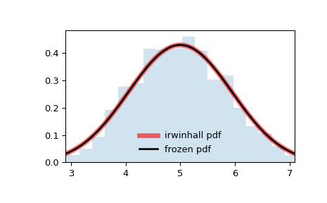
Display the probability density function (
pdf):>>> x = np.linspace(irwinhall.ppf(0.01, n), ... irwinhall.ppf(0.99, n), 100) >>> ax.plot(x, irwinhall.pdf(x, n), ... 'r-', lw=5, alpha=0.6, label='irwinhall pdf')
Alternatively, the distribution object can be called (as a function) to fix the shape, location and scale parameters. This returns a “frozen” RV object holding the given parameters fixed.
Freeze the distribution and display the frozen
pdf:>>> rv = irwinhall(n) >>> ax.plot(x, rv.pdf(x), 'k-', lw=2, label='frozen pdf')
Check accuracy of
cdfandppf:>>> vals = irwinhall.ppf([0.001, 0.5, 0.999], n) >>> np.allclose([0.001, 0.5, 0.999], irwinhall.cdf(vals, n)) True
Generate random numbers:
>>> r = irwinhall.rvs(n, size=1000)
And compare the histogram:
>>> ax.hist(r, density=True, bins='auto', histtype='stepfilled', alpha=0.2)
>>> ax.set_xlim([x[0], x[-1]])
>>> ax.legend(loc='best', frameon=False)
>>> plt.show()
