scipy.interpolate.

BarycentricInterpolator

class scipy.interpolate.BarycentricInterpolator(xi, yi=None, axis=0, *, wi=None, random_state=None)

Interpolating polynomial for a set of points.

Constructs a polynomial that passes through a given set of points. Allows evaluation of the polynomial and all its derivatives, efficient changing of the y-values to be interpolated, and updating by adding more x- and y-values.

For reasons of numerical stability, this function does not compute the coefficients of the polynomial.

The values yi need to be provided before the function is evaluated, but none of the preprocessing depends on them, so rapid updates are possible.

Parameters:

xiarray_like, shape (npoints, )

1-D array of x coordinates of the points the polynomial should pass through

yiarray_like, shape (…, npoints, …), optional

N-D array of y coordinates of the points the polynomial should pass through. If None, the y values will be supplied later via the set_y method. The length of yi along the interpolation axis must be equal to the length of xi. Use the axis parameter to select correct axis.

axisint, optional

Axis in the yi array corresponding to the x-coordinate values. Defaults to axis=0.

wiarray_like, optional

The barycentric weights for the chosen interpolation points xi. If absent or None, the weights will be computed from xi (default). This allows for the reuse of the weights wi if several interpolants are being calculated using the same nodes xi, without re-computation.

random_state{None, int, numpy.random.Generator, numpy.random.RandomState}, optional

If seed is None (or np.random), the numpy.random.RandomState singleton is used. If seed is an int, a new RandomState instance is used, seeded with seed. If seed is already a Generator or RandomState instance then that instance is used.

Attributes:

dtype

Methods

__call__(x)	Evaluate the interpolating polynomial at the points x
add_xi(xi[, yi])	Add more x values to the set to be interpolated
derivative(x[, der])	Evaluate a single derivative of the polynomial at the point x.
derivatives(x[, der])	Evaluate several derivatives of the polynomial at the point x
set_yi(yi[, axis])	Update the y values to be interpolated

Notes

This class uses a “barycentric interpolation” method that treats the problem as a special case of rational function interpolation. This algorithm is quite stable, numerically, but even in a world of exact computation, unless the x coordinates are chosen very carefully - Chebyshev zeros (e.g., cos(i*pi/n)) are a good choice - polynomial interpolation itself is a very ill-conditioned process due to the Runge phenomenon.

Based on Berrut and Trefethen 2004, “Barycentric Lagrange Interpolation”.

Examples

Try it in your browser!

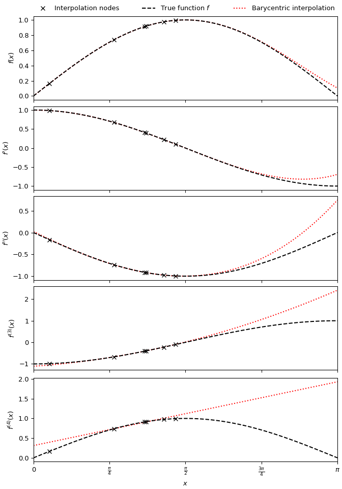
To produce a quintic barycentric interpolant approximating the function \(\sin x\), and its first four derivatives, using six randomly-spaced nodes in \((0, \frac{\pi}{2})\):

>>> import numpy as np
>>> import matplotlib.pyplot as plt
>>> from scipy.interpolate import BarycentricInterpolator
>>> rng = np.random.default_rng()
>>> xi = rng.random(6) * np.pi/2
>>> f, f_d1, f_d2, f_d3, f_d4 = np.sin, np.cos, lambda x: -np.sin(x), lambda x: -np.cos(x), np.sin
>>> P = BarycentricInterpolator(xi, f(xi), random_state=rng)
>>> fig, axs = plt.subplots(5, 1, sharex=True, layout='constrained', figsize=(7,10))
>>> x = np.linspace(0, np.pi, 100)
>>> axs[0].plot(x, P(x), 'r:', x, f(x), 'k--', xi, f(xi), 'xk')
>>> axs[1].plot(x, P.derivative(x), 'r:', x, f_d1(x), 'k--', xi, f_d1(xi), 'xk')
>>> axs[2].plot(x, P.derivative(x, 2), 'r:', x, f_d2(x), 'k--', xi, f_d2(xi), 'xk')
>>> axs[3].plot(x, P.derivative(x, 3), 'r:', x, f_d3(x), 'k--', xi, f_d3(xi), 'xk')
>>> axs[4].plot(x, P.derivative(x, 4), 'r:', x, f_d4(x), 'k--', xi, f_d4(xi), 'xk')
>>> axs[0].set_xlim(0, np.pi)
>>> axs[4].set_xlabel(r"$x$")
>>> axs[4].set_xticks([i * np.pi / 4 for i in range(5)],
...                   ["0", r"$\frac{\pi}{4}$", r"$\frac{\pi}{2}$", r"$\frac{3\pi}{4}$", r"$\pi$"])
>>> axs[0].set_ylabel("$f(x)$")
>>> axs[1].set_ylabel("$f'(x)$")
>>> axs[2].set_ylabel("$f''(x)$")
>>> axs[3].set_ylabel("$f^{(3)}(x)$")
>>> axs[4].set_ylabel("$f^{(4)}(x)$")
>>> labels = ['Interpolation nodes', 'True function $f$', 'Barycentric interpolation']
>>> axs[0].legend(axs[0].get_lines()[::-1], labels, bbox_to_anchor=(0., 1.02, 1., .102),
...               loc='lower left', ncols=3, mode="expand", borderaxespad=0., frameon=False)
>>> plt.show()

Go BackOpen In Tab