scipy.stats.

kurtosis#

scipy.stats.kurtosis(a, axis=0, fisher=True, bias=True, nan_policy='propagate', *, keepdims=False)[source]#

Compute the kurtosis (Fisher or Pearson) of a dataset.

Kurtosis is the fourth central moment divided by the square of the variance. If Fisher’s definition is used, then 3.0 is subtracted from the result to give 0.0 for a normal distribution.

If bias is False then the kurtosis is calculated using k statistics to eliminate bias coming from biased moment estimators

Use kurtosistest to see if result is close enough to normal.

Parameters:

aarray

Data for which the kurtosis is calculated.

axisint or None, default: 0

If an int, the axis of the input along which to compute the statistic. The statistic of each axis-slice (e.g. row) of the input will appear in a corresponding element of the output. If None, the input will be raveled before computing the statistic.

fisherbool, optional

If True, Fisher’s definition is used (normal ==> 0.0). If False, Pearson’s definition is used (normal ==> 3.0).

biasbool, optional

If False, then the calculations are corrected for statistical bias.

nan_policy{‘propagate’, ‘omit’, ‘raise’}

Defines how to handle input NaNs.

propagate: if a NaN is present in the axis slice (e.g. row) along which the statistic is computed, the corresponding entry of the output will be NaN.
omit: NaNs will be omitted when performing the calculation. If insufficient data remains in the axis slice along which the statistic is computed, the corresponding entry of the output will be NaN.
raise: if a NaN is present, a ValueError will be raised.

keepdimsbool, default: False

If this is set to True, the axes which are reduced are left in the result as dimensions with size one. With this option, the result will broadcast correctly against the input array.

Returns:

kurtosisarray: The kurtosis of values along an axis, returning NaN where all values are equal.

Notes

Beginning in SciPy 1.9, np.matrix inputs (not recommended for new code) are converted to np.ndarray before the calculation is performed. In this case, the output will be a scalar or np.ndarray of appropriate shape rather than a 2D np.matrix. Similarly, while masked elements of masked arrays are ignored, the output will be a scalar or np.ndarray rather than a masked array with mask=False.

References

[1]

Zwillinger, D. and Kokoska, S. (2000). CRC Standard Probability and Statistics Tables and Formulae. Chapman & Hall: New York. 2000.

Examples

In Fisher’s definition, the kurtosis of the normal distribution is zero. In the following example, the kurtosis is close to zero, because it was calculated from the dataset, not from the continuous distribution.

>>> import numpy as np
>>> from scipy.stats import norm, kurtosis
>>> data = norm.rvs(size=1000, random_state=3)
>>> kurtosis(data)
-0.06928694200380558

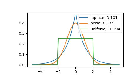
The distribution with a higher kurtosis has a heavier tail. The zero valued kurtosis of the normal distribution in Fisher’s definition can serve as a reference point.

>>> import matplotlib.pyplot as plt
>>> import scipy.stats as stats
>>> from scipy.stats import kurtosis

>>> x = np.linspace(-5, 5, 100)
>>> ax = plt.subplot()
>>> distnames = ['laplace', 'norm', 'uniform']

>>> for distname in distnames:
...     if distname == 'uniform':
...         dist = getattr(stats, distname)(loc=-2, scale=4)
...     else:
...         dist = getattr(stats, distname)
...     data = dist.rvs(size=1000)
...     kur = kurtosis(data, fisher=True)
...     y = dist.pdf(x)
...     ax.plot(x, y, label="{}, {}".format(distname, round(kur, 3)))
...     ax.legend()

The Laplace distribution has a heavier tail than the normal distribution. The uniform distribution (which has negative kurtosis) has the thinnest tail.

../../_images/scipy-stats-kurtosis-1.png