scipy.stats.

gzscore

scipy.stats.gzscore(a, *, axis=0, ddof=0, nan_policy='propagate')

Compute the geometric standard score.

Compute the geometric z score of each strictly positive value in the sample, relative to the geometric mean and standard deviation. Mathematically the geometric z score can be evaluated as:

gzscore = log(a/gmu) / log(gsigma)

where gmu (resp. gsigma) is the geometric mean (resp. standard deviation).

Parameters:

aarray_like

Sample data.

axisint or None, optional

Axis along which to operate. Default is 0. If None, compute over the whole array a.

ddofint, optional

Degrees of freedom correction in the calculation of the standard deviation. Default is 0.

nan_policy{‘propagate’, ‘raise’, ‘omit’}, optional

Defines how to handle when input contains nan. ‘propagate’ returns nan, ‘raise’ throws an error, ‘omit’ performs the calculations ignoring nan values. Default is ‘propagate’. Note that when the value is ‘omit’, nans in the input also propagate to the output, but they do not affect the geometric z scores computed for the non-nan values.

Returns:

gzscorearray_like

The geometric z scores, standardized by geometric mean and geometric standard deviation of input array a.

See also

gmean

Geometric mean

gstd

Geometric standard deviation

zscore

Standard score

Notes

This function preserves ndarray subclasses, and works also with matrices and masked arrays (it uses asanyarray instead of asarray for parameters).

Added in version 1.8.

References

[1]

“Geometric standard score”, Wikipedia, https://en.wikipedia.org/wiki/Geometric_standard_deviation#Geometric_standard_score.

Examples

Try it in your browser!

Draw samples from a log-normal distribution:

>>> import numpy as np
>>> from scipy.stats import zscore, gzscore
>>> import matplotlib.pyplot as plt

>>> rng = np.random.default_rng()
>>> mu, sigma = 3., 1.  # mean and standard deviation
>>> x = rng.lognormal(mu, sigma, size=500)

Display the histogram of the samples:

>>> fig, ax = plt.subplots()
>>> ax.hist(x, 50)
>>> plt.show()

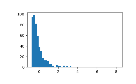
Display the histogram of the samples standardized by the classical zscore. Distribution is rescaled but its shape is unchanged.

>>> fig, ax = plt.subplots()
>>> ax.hist(zscore(x), 50)
>>> plt.show()

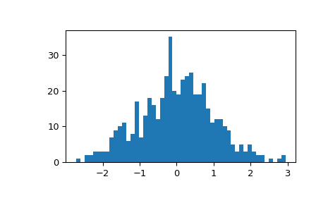
Demonstrate that the distribution of geometric zscores is rescaled and quasinormal:

>>> fig, ax = plt.subplots()
>>> ax.hist(gzscore(x), 50)
>>> plt.show()

Go BackOpen In Tab