scipy.special.shichi#

scipy.special.shichi(x, out=None) = <ufunc 'shichi'>#

Hyperbolic sine and cosine integrals.

The hyperbolic sine integral is

\[\int_0^x \frac{\sinh{t}}{t}dt\]

and the hyperbolic cosine integral is

\[\gamma + \log(x) + \int_0^x \frac{\cosh{t} - 1}{t} dt\]

where \(\gamma\) is Euler’s constant and \(\log\) is the principal branch of the logarithm [1].

Parameters:

xarray_like: Real or complex points at which to compute the hyperbolic sine and cosine integrals.
outtuple of ndarray, optional: Optional output arrays for the function results

Returns:

siscalar or ndarray: Hyperbolic sine integral at x
ciscalar or ndarray: Hyperbolic cosine integral at x

See also

sici: Sine and cosine integrals.
exp1: Exponential integral E1.
expi: Exponential integral Ei.

Notes

For real arguments with x < 0, chi is the real part of the hyperbolic cosine integral. For such points chi(x) and chi(x + 0j) differ by a factor of 1j*pi.

For real arguments the function is computed by calling Cephes’ [2] shichi routine. For complex arguments the algorithm is based on Mpmath’s [3] shi and chi routines.

References

[1]

Milton Abramowitz and Irene A. Stegun, eds. Handbook of Mathematical Functions with Formulas, Graphs, and Mathematical Tables. New York: Dover, 1972. (See Section 5.2.)

[2]

Cephes Mathematical Functions Library, http://www.netlib.org/cephes/

[3]

Fredrik Johansson and others. “mpmath: a Python library for arbitrary-precision floating-point arithmetic” (Version 0.19) http://mpmath.org/

Examples

>>> import numpy as np
>>> import matplotlib.pyplot as plt
>>> from scipy.special import shichi, sici

shichi accepts real or complex input:

>>> shichi(0.5)
(0.5069967498196671, -0.05277684495649357)
>>> shichi(0.5 + 2.5j)
((0.11772029666668238+1.831091777729851j),
 (0.29912435887648825+1.7395351121166562j))

The hyperbolic sine and cosine integrals Shi(z) and Chi(z) are related to the sine and cosine integrals Si(z) and Ci(z) by

Shi(z) = -i*Si(i*z)
Chi(z) = Ci(-i*z) + i*pi/2

>>> z = 0.25 + 5j
>>> shi, chi = shichi(z)
>>> shi, -1j*sici(1j*z)[0]            # Should be the same.
((-0.04834719325101729+1.5469354086921228j),
 (-0.04834719325101729+1.5469354086921228j))
>>> chi, sici(-1j*z)[1] + 1j*np.pi/2  # Should be the same.
((-0.19568708973868087+1.556276312103824j),
 (-0.19568708973868087+1.556276312103824j))

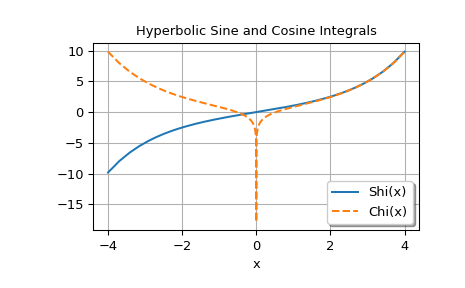
Plot the functions evaluated on the real axis:

>>> xp = np.geomspace(1e-8, 4.0, 250)
>>> x = np.concatenate((-xp[::-1], xp))
>>> shi, chi = shichi(x)

>>> fig, ax = plt.subplots()
>>> ax.plot(x, shi, label='Shi(x)')
>>> ax.plot(x, chi, '--', label='Chi(x)')
>>> ax.set_xlabel('x')
>>> ax.set_title('Hyperbolic Sine and Cosine Integrals')
>>> ax.legend(shadow=True, framealpha=1, loc='lower right')
>>> ax.grid(True)
>>> plt.show()

../../_images/scipy-special-shichi-1.png