exponential#
- scipy.signal.windows.exponential(M, center=None, tau=1.0, sym=True, *, xp=None, device=None)[source]#
Return an exponential (or Poisson) window.
- Parameters:
- Mint
Number of points in the output window. If zero, an empty array is returned. An exception is thrown when it is negative.
- centerfloat, optional
Parameter defining the center location of the window function. The default value if not given is
center = (M-1) / 2. This parameter must take its default value for symmetric windows.- taufloat, optional
Parameter defining the decay. For
center = 0usetau = -(M-1) / ln(x)ifxis the fraction of the window remaining at the end.- symbool, optional
When True (default), generates a symmetric window, for use in filter design. When False, generates a periodic window, for use in spectral analysis.
- xparray_namespace, optional
Optional array namespace. Should be compatible with the array API standard, or supported by array-api-compat. Default:
numpy- deviceany
optional device specification for output. Should match one of the supported device specification in
xp.
- Returns:
- wndarray
The window, with the maximum value normalized to 1 (though the value 1 does not appear if M is even and sym is True).
Notes
The Exponential window is defined as
\[w(n) = e^{-|n-center| / \tau}\]Array API Standard Support
exponentialhas experimental support for Python Array API Standard compatible backends in addition to NumPy. Please consider testing these features by setting an environment variableSCIPY_ARRAY_API=1and providing CuPy, PyTorch, JAX, or Dask arrays as array arguments. The following combinations of backend and device (or other capability) are supported.Library
CPU
GPU
NumPy
✅
n/a
CuPy
n/a
✅
PyTorch
✅
✅
JAX
✅
✅
Dask
✅
n/a
See Support for the array API standard for more information.
References
[1]S. Gade and H. Herlufsen, “Windows to FFT analysis (Part I)”, Technical Review 3, Bruel & Kjaer, 1987.
Examples
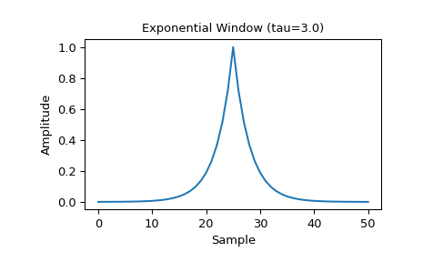
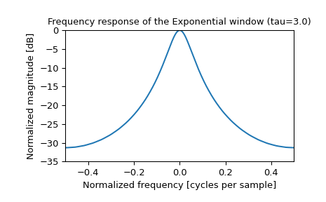
Plot the symmetric window and its frequency response:
>>> import numpy as np
>>> from scipy import signal
>>> from scipy.fft import fft, fftshift
>>> import matplotlib.pyplot as plt
>>> M = 51
>>> tau = 3.0
>>> window = signal.windows.exponential(M, tau=tau)
>>> plt.plot(window)
>>> plt.title("Exponential Window (tau=3.0)")
>>> plt.ylabel("Amplitude")
>>> plt.xlabel("Sample")
>>> plt.figure()
>>> A = fft(window, 2048) / (len(window)/2.0)
>>> freq = np.linspace(-0.5, 0.5, len(A))
>>> response = 20 * np.log10(np.abs(fftshift(A / abs(A).max())))
>>> plt.plot(freq, response)
>>> plt.axis([-0.5, 0.5, -35, 0])
>>> plt.title("Frequency response of the Exponential window (tau=3.0)")
>>> plt.ylabel("Normalized magnitude [dB]")
>>> plt.xlabel("Normalized frequency [cycles per sample]")
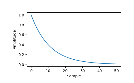
This function can also generate non-symmetric windows:
>>> tau2 = -(M-1) / np.log(0.01)
>>> window2 = signal.windows.exponential(M, 0, tau2, False)
>>> plt.figure()
>>> plt.plot(window2)
>>> plt.ylabel("Amplitude")
>>> plt.xlabel("Sample")