__call__#
- LSQSphereBivariateSpline.__call__(theta, phi, dtheta=0, dphi=0, grid=True)[source]#
Evaluate the spline or its derivatives at given positions.
- Parameters:
- theta, phiarray_like
Input coordinates.
If grid is False, evaluate the spline at points
(theta[i], phi[i]), i=0, ..., len(x)-1. Standard Numpy broadcasting is obeyed.If grid is True: evaluate spline at the grid points defined by the coordinate arrays theta, phi. The arrays must be sorted to increasing order. The ordering of axes is consistent with
np.meshgrid(..., indexing="ij")and inconsistent with the default orderingnp.meshgrid(..., indexing="xy").- dthetaint, optional
Order of theta-derivative
Added in version 0.14.0.
- dphiint
Order of phi-derivative
Added in version 0.14.0.
- gridbool
Whether to evaluate the results on a grid spanned by the input arrays, or at points specified by the input arrays.
Added in version 0.14.0.
Examples
Suppose that we want to use splines to interpolate a bivariate function on a sphere. The value of the function is known on a grid of longitudes and colatitudes.
>>> import numpy as np
>>> from scipy.interpolate import RectSphereBivariateSpline
>>> def f(theta, phi):
...     return np.sin(theta) * np.cos(phi)
We evaluate the function on the grid. Note that the default indexing=”xy” of meshgrid would result in an unexpected (transposed) result after interpolation.
>>> thetaarr = np.linspace(0, np.pi, 22)[1:-1]
>>> phiarr = np.linspace(0, 2 * np.pi, 21)[:-1]
>>> thetagrid, phigrid = np.meshgrid(thetaarr, phiarr, indexing="ij")
>>> zdata = f(thetagrid, phigrid)
We next set up the interpolator and use it to evaluate the function on a finer grid.
>>> rsbs = RectSphereBivariateSpline(thetaarr, phiarr, zdata)
>>> thetaarr_fine = np.linspace(0, np.pi, 200)
>>> phiarr_fine = np.linspace(0, 2 * np.pi, 200)
>>> zdata_fine = rsbs(thetaarr_fine, phiarr_fine)
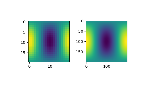
Finally we plot the coarsly-sampled input data alongside the finely-sampled interpolated data to check that they agree.
>>> import matplotlib.pyplot as plt
>>> fig = plt.figure()
>>> ax1 = fig.add_subplot(1, 2, 1)
>>> ax2 = fig.add_subplot(1, 2, 2)
>>> ax1.imshow(zdata)
>>> ax2.imshow(zdata_fine)
>>> plt.show()