fht#
- scipy.fft.fht(a, dln, mu, offset=0.0, bias=0.0)[source]#
Compute the fast Hankel transform.
Computes the discrete Hankel transform of a logarithmically spaced periodic sequence using the FFTLog algorithm [1], [2].
- Parameters:
- aarray_like (…, n)
Real periodic input array, uniformly logarithmically spaced. For multidimensional input, the transform is performed over the last axis.
- dlnfloat
Uniform logarithmic spacing of the input array.
- mufloat
Order of the Hankel transform, any positive or negative real number.
- offsetfloat, optional
Offset of the uniform logarithmic spacing of the output array.
- biasfloat, optional
Exponent of power law bias, any positive or negative real number.
- Returns:
- Aarray_like (…, n)
The transformed output array, which is real, periodic, uniformly logarithmically spaced, and of the same shape as the input array.
Notes
This function computes a discrete version of the Hankel transform
\[A(k) = \int_{0}^{\infty} \! a(r) \, J_\mu(kr) \, k \, dr \;,\]where \(J_\mu\) is the Bessel function of order \(\mu\). The index \(\mu\) may be any real number, positive or negative. Note that the numerical Hankel transform uses an integrand of \(k \, dr\), while the mathematical Hankel transform is commonly defined using \(r \, dr\).
The input array a is a periodic sequence of length \(n\), uniformly logarithmically spaced with spacing dln,
\[a_j = a(r_j) \;, \quad r_j = r_c \exp[(j-j_c) \, \mathtt{dln}]\]centred about the point \(r_c\). Note that the central index \(j_c = (n-1)/2\) is half-integral if \(n\) is even, so that \(r_c\) falls between two input elements. Similarly, the output array A is a periodic sequence of length \(n\), also uniformly logarithmically spaced with spacing dln
\[A_j = A(k_j) \;, \quad k_j = k_c \exp[(j-j_c) \, \mathtt{dln}]\]centred about the point \(k_c\).
The centre points \(r_c\) and \(k_c\) of the periodic intervals may be chosen arbitrarily, but it would be usual to choose the product \(k_c r_c = k_j r_{n-1-j} = k_{n-1-j} r_j\) to be unity. This can be changed using the offset parameter, which controls the logarithmic offset \(\log(k_c) = \mathtt{offset} - \log(r_c)\) of the output array. Choosing an optimal value for offset may reduce ringing of the discrete Hankel transform.
If the bias parameter is nonzero, this function computes a discrete version of the biased Hankel transform
\[A(k) = \int_{0}^{\infty} \! a_q(r) \, (kr)^q \, J_\mu(kr) \, k \, dr\]where \(q\) is the value of bias, and a power law bias \(a_q(r) = a(r) \, (kr)^{-q}\) is applied to the input sequence. Biasing the transform can help approximate the continuous transform of \(a(r)\) if there is a value \(q\) such that \(a_q(r)\) is close to a periodic sequence, in which case the resulting \(A(k)\) will be close to the continuous transform.
Array API Standard Support
fhthas experimental support for Python Array API Standard compatible backends in addition to NumPy. Please consider testing these features by setting an environment variableSCIPY_ARRAY_API=1and providing CuPy, PyTorch, JAX, or Dask arrays as array arguments. The following combinations of backend and device (or other capability) are supported.Library
CPU
GPU
NumPy
✅
n/a
CuPy
n/a
✅
PyTorch
✅
✅
JAX
✅
✅
Dask
⚠️ computes graph
n/a
See Support for the array API standard for more information.
References
[1]Talman J. D., 1978, J. Comp. Phys., 29, 35
Examples
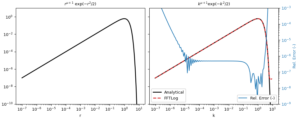
This example is the adapted version of
fftlogtest.fwhich is provided in [2]. It evaluates the integral\[\int^\infty_0 r^{\mu+1} \exp(-r^2/2) J_\mu(kr) k dr = k^{\mu+1} \exp(-k^2/2) .\]>>> import numpy as np >>> from scipy import fft >>> import matplotlib.pyplot as plt
Parameters for the transform.
>>> mu = 0.0                     # Order mu of Bessel function
>>> r = np.logspace(-7, 1, 128)  # Input evaluation points
>>> dln = np.log(r[1]/r[0])      # Step size
>>> offset = fft.fhtoffset(dln, initial=-6*np.log(10), mu=mu)
>>> k = np.exp(offset)/r[::-1]   # Output evaluation points
Define the analytical function.
>>> def f(x, mu):
...     """Analytical function: x^(mu+1) exp(-x^2/2)."""
...     return x**(mu + 1)*np.exp(-x**2/2)
Evaluate the function at
rand compute the corresponding values atkusing FFTLog.>>> a_r = f(r, mu) >>> fht = fft.fht(a_r, dln, mu=mu, offset=offset)
For this example we can actually compute the analytical response (which in this case is the same as the input function) for comparison and compute the relative error.
>>> a_k = f(k, mu)
>>> rel_err = abs((fht-a_k)/a_k)
Plot the result.
>>> figargs = {'sharex': True, 'sharey': True, 'constrained_layout': True}
>>> fig, (ax1, ax2) = plt.subplots(1, 2, figsize=(10, 4), **figargs)
>>> ax1.set_title(r'$r^{\mu+1}\ \exp(-r^2/2)$')
>>> ax1.loglog(r, a_r, 'k', lw=2)
>>> ax1.set_xlabel('r')
>>> ax2.set_title(r'$k^{\mu+1} \exp(-k^2/2)$')
>>> ax2.loglog(k, a_k, 'k', lw=2, label='Analytical')
>>> ax2.loglog(k, fht, 'C3--', lw=2, label='FFTLog')
>>> ax2.set_xlabel('k')
>>> ax2.legend(loc=3, framealpha=1)
>>> ax2.set_ylim([1e-10, 1e1])
>>> ax2b = ax2.twinx()
>>> ax2b.loglog(k, rel_err, 'C0', label='Rel. Error (-)')
>>> ax2b.set_ylabel('Rel. Error (-)', color='C0')
>>> ax2b.tick_params(axis='y', labelcolor='C0')
>>> ax2b.legend(loc=4, framealpha=1)
>>> ax2b.set_ylim([1e-9, 1e-3])
>>> plt.show()