1-D interpolation#
Piecewise linear interpolation#
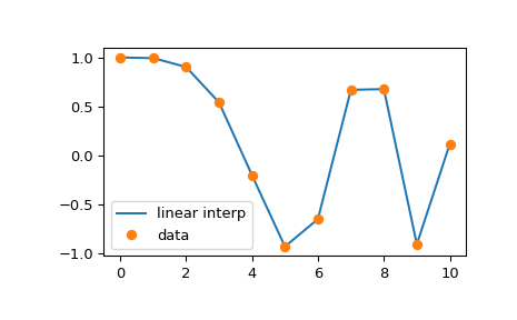
If all you need is a linear (a.k.a. broken line) interpolation, you can use
the numpy.interp routine. It takes two arrays of data to interpolate, x,
and y, and a third array, xnew, of points to evaluate the interpolation on:
>>> import numpy as np
>>> x = np.linspace(0, 10, num=11)
>>> y = np.cos(-x**2 / 9.0)
Construct the interpolation
>>> xnew = np.linspace(0, 10, num=1001)
>>> ynew = np.interp(xnew, x, y)
And plot it
>>> import matplotlib.pyplot as plt
>>> plt.plot(xnew, ynew, '-', label='linear interp')
>>> plt.plot(x, y, 'o', label='data')
>>> plt.legend(loc='best')
>>> plt.show()
Cubic splines#
Of course, piecewise linear interpolation produces corners at data points,
where linear pieces join. To produce a smoother curve, you can use cubic
splines, where the interpolating curve is made of cubic pieces with matching
first and second derivatives. In code, these objects are represented via the
CubicSpline class instances. An instance is constructed with the x and
y arrays of data, and then it can be evaluated using the target xnew
values:
>>> from scipy.interpolate import CubicSpline
>>> spl = CubicSpline([1, 2, 3, 4, 5, 6], [1, 4, 8, 16, 25, 36])
>>> spl(2.5)
5.57
A CubicSpline object’s __call__ method accepts both scalar values and
arrays. It also accepts a second argument, nu, to evaluate the
derivative of order nu. As an example, we plot the derivatives of a spline:
>>> from scipy.interpolate import CubicSpline
>>> x = np.linspace(0, 10, num=11)
>>> y = np.cos(-x**2 / 9.)
>>> spl = CubicSpline(x, y)
>>> import matplotlib.pyplot as plt
>>> fig, ax = plt.subplots(4, 1, figsize=(5, 7))
>>> xnew = np.linspace(0, 10, num=1001)
>>> ax[0].plot(xnew, spl(xnew))
>>> ax[0].plot(x, y, 'o', label='data')
>>> ax[1].plot(xnew, spl(xnew, nu=1), '--', label='1st derivative')
>>> ax[2].plot(xnew, spl(xnew, nu=2), '--', label='2nd derivative')
>>> ax[3].plot(xnew, spl(xnew, nu=3), '--', label='3rd derivative')
>>> for j in range(4):
...     ax[j].legend(loc='best')
>>> plt.tight_layout()
>>> plt.show()
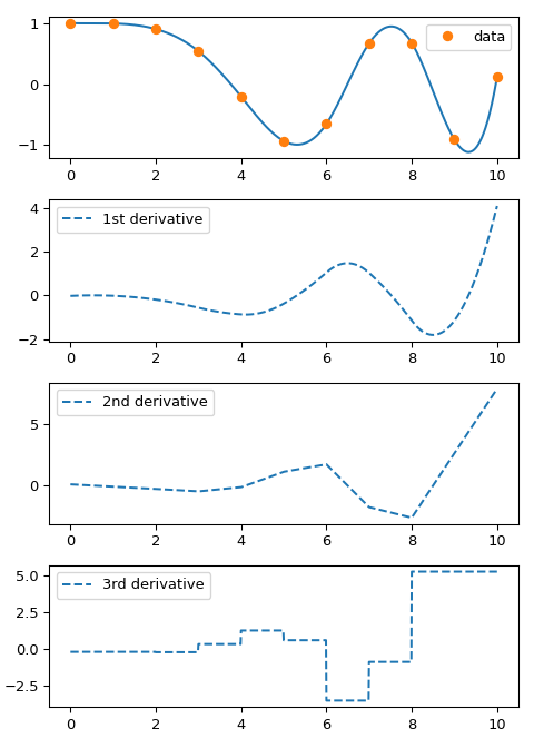
Note that the first and second derivatives are continuous by construction, and the third derivative jumps at data points.
Monotone interpolants#
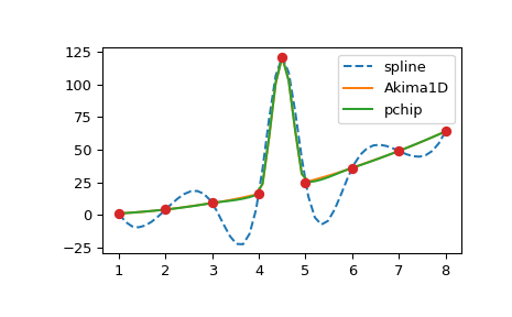
Cubic splines are by construction twice continuously differentiable. This may
lead to the spline function oscillating and ‘’overshooting’’ in between the
data points. In these situations, an alternative is to use the so-called
monotone cubic interpolants: these are constructed to be only once
continuously differentiable, and attempt to preserve the local shape implied
by the data. scipy.interpolate provides two objects of this kind:
PchipInterpolator and Akima1DInterpolator . To illustrate, let’s consider
data with an outlier:
>>> from scipy.interpolate import CubicSpline, PchipInterpolator, Akima1DInterpolator
>>> x = np.array([1., 2., 3., 4., 4.5, 5., 6., 7., 8])
>>> y = x**2
>>> y[4] += 101
>>> import matplotlib.pyplot as plt
>>> xx = np.linspace(1, 8, 51)
>>> plt.plot(xx, CubicSpline(x, y)(xx), '--', label='spline')
>>> plt.plot(xx, Akima1DInterpolator(x, y)(xx), '-', label='Akima1D')
>>> plt.plot(xx, PchipInterpolator(x, y)(xx), '-', label='pchip')
>>> plt.plot(x, y, 'o')
>>> plt.legend()
>>> plt.show()
Interpolation with B-splines#
B-splines form an alternative (if formally equivalent) representation of piecewise polynomials. This basis is generally more computationally stable than the power basis and is useful for a variety of applications which include interpolation, regression and curve representation. Details are given in the piecewise polynomials section, and here we illustrate their usage by constructing the interpolation of a sine function:
>>> x = np.linspace(0, 3/2, 7)
>>> y = np.sin(np.pi*x)
To construct the interpolating objects given data arrays, x and y,
we use the make_interp_spline function:
>>> from scipy.interpolate import make_interp_spline
>>> bspl = make_interp_spline(x, y, k=3)
This function returns an object which has an interface similar to that
of the CubicSpline objects. In particular, it can be evaluated at a data
point and differentiated:
>>> der = bspl.derivative()      # a BSpline representing the derivative
>>> import matplotlib.pyplot as plt
>>> xx = np.linspace(0, 3/2, 51)
>>> plt.plot(xx, bspl(xx), '--', label=r'$\sin(\pi x)$ approx')
>>> plt.plot(x, y, 'o', label='data')
>>> plt.plot(xx, der(xx)/np.pi, '--', label='$d \sin(\pi x)/dx / \pi$ approx')
>>> plt.legend()
>>> plt.show()
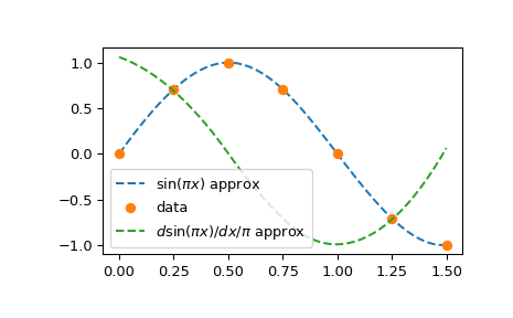
Note that by specifying k=3 in the make_interp_spline call, we requested
a cubic spline (this is the default, so k=3 could have been omitted); the
derivative of a cubic is a quadratic:
>>> bspl.k, der.k
(3, 2)
By default, the result of make_interp_spline(x, y) is equivalent to
CubicSpline(x, y). The difference is that the former allows several optional
capabilities: it can construct splines of various degrees (via the optional
argument k) and predefined knots (via the optional argument t).
Boundary conditions for the spline interpolation can be controlled by
the bc_type argument to make_interp_spline function and CubicSpline
constructor. By default, both use the ‘not-a-knot’ boundary
condition.
Parametric spline curves#
So far we considered spline functions, where the data, y, is expected to
depend explicitly on the independent variable x—so that the interpolating
function satisfies \(f(x_j) = y_j\). Spline curves treat
the x and y arrays as coordinates of points, \(\mathbf{p}_j\) on a
plane, and an interpolating curve which passes through these points is
parameterized by some additional parameter (typically called u). Note that
this construction readily generalizes to higher dimensions where
\(\mathbf{p}_j\) are points in an N-dimensional space.
Spline curves can be easily constructed using the fact that interpolation
functions handle multidimensional data arrays. The values of the parameter
u, corresponding to the data points, need to be separately supplied
by the user.
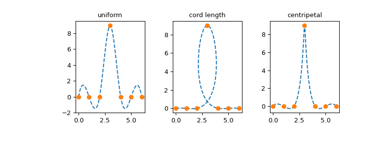
The choice of parametrization is problem-dependent and different parametrizations
may produce vastly different curves. As an example, we consider three
parametrizations of (a somewhat difficult) dataset, which we take from
Chapter 6 of Ref [1] listed in the BSpline docstring:
>>> x = [0, 1, 2, 3, 4, 5, 6]
>>> y = [0, 0, 0, 9, 0, 0, 0]
>>> p = np.stack((x, y))
>>> p
array([[0, 1, 2, 3, 4, 5, 6],
       [0, 0, 0, 9, 0, 0, 0]])
We take elements of the p array as coordinates of seven points on the
plane, where p[:, j] gives the coordinates of the point
\(\mathbf{p}_j\).
First, consider the uniform parametrization, \(u_j = j\):
>>> u_unif = x
Second, we consider the so-called cord length parametrization, which is nothing but a cumulative length of straight line segments connecting the data points:
for \(j=1, 2, \dots\) and \(u_0 = 0\). Here \(| \cdots |\) is the length between the consecutive points \(p_j\) on the plane.
>>> dp = p[:, 1:] - p[:, :-1]      # 2-vector distances between points
>>> l = (dp**2).sum(axis=0)        # squares of lengths of 2-vectors between points
>>> u_cord = np.sqrt(l).cumsum()   # cumulative sums of 2-norms
>>> u_cord = np.r_[0, u_cord]      # the first point is parameterized at zero
Finally, we consider what is sometimes called the centripetal parametrization: \(u_j = u_{j-1} + |\mathbf{p}_j - \mathbf{p}_{j-1}|^{1/2}\). Due to the extra square root, the difference between consecutive values \(u_j - u_{j-1}\) will be smaller than for the cord length parametrization:
>>> u_c = np.r_[0, np.cumsum((dp**2).sum(axis=0)**0.25)]
Now plot the resulting curves:
>>> from scipy.interpolate import make_interp_spline
>>> import matplotlib.pyplot as plt
>>> fig, ax = plt.subplots(1, 3, figsize=(8, 3))
>>> parametrizations = ['uniform', 'cord length', 'centripetal']
>>>
>>> for j, u in enumerate([u_unif, u_cord, u_c]):
...    spl = make_interp_spline(u, p, axis=1)    # note p is a 2D array
...
...    uu = np.linspace(u[0], u[-1], 51)
...    xx, yy = spl(uu)
...
...    ax[j].plot(xx, yy, '--')
...    ax[j].plot(p[0, :], p[1, :], 'o')
...    ax[j].set_title(parametrizations[j])
>>> plt.show()
Legacy interface for 1-D interpolation (interp1d)#
Note
interp1d is considered legacy API and is not recommended for use in new
code. Consider using more specific interpolators instead.
The interp1d class in scipy.interpolate is a convenient method to
create a function based on fixed data points, which can be evaluated
anywhere within the domain defined by the given data using linear
interpolation. An instance of this class is created by passing the 1-D
vectors comprising the data. The instance of this class defines a
__call__ method and can therefore be treated like a function which
interpolates between known data values to obtain unknown values.
Behavior at the boundary can be
specified at instantiation time. The following example demonstrates
its use, for linear and cubic spline interpolation:
>>> from scipy.interpolate import interp1d
>>> x = np.linspace(0, 10, num=11, endpoint=True)
>>> y = np.cos(-x**2/9.0)
>>> f = interp1d(x, y)
>>> f2 = interp1d(x, y, kind='cubic')
>>> xnew = np.linspace(0, 10, num=41, endpoint=True)
>>> import matplotlib.pyplot as plt
>>> plt.plot(x, y, 'o', xnew, f(xnew), '-', xnew, f2(xnew), '--')
>>> plt.legend(['data', 'linear', 'cubic'], loc='best')
>>> plt.show()
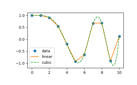
The ‘cubic’ kind of interp1d is equivalent to make_interp_spline, and
the ‘linear’ kind is equivalent to numpy.interp while also allowing
N-dimensional y arrays.
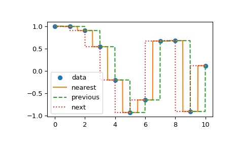
Another set of interpolations in interp1d is nearest, previous, and
next, where they return the nearest, previous, or next point along the
x-axis. Nearest and next can be thought of as a special case of a causal
interpolating filter. The following example demonstrates their use, using the
same data as in the previous example:
>>> from scipy.interpolate import interp1d
>>> x = np.linspace(0, 10, num=11, endpoint=True)
>>> y = np.cos(-x**2/9.0)
>>> f1 = interp1d(x, y, kind='nearest')
>>> f2 = interp1d(x, y, kind='previous')
>>> f3 = interp1d(x, y, kind='next')
>>> xnew = np.linspace(0, 10, num=1001, endpoint=True)
>>> import matplotlib.pyplot as plt
>>> plt.plot(x, y, 'o')
>>> plt.plot(xnew, f1(xnew), '-', xnew, f2(xnew), '--', xnew, f3(xnew), ':')
>>> plt.legend(['data', 'nearest', 'previous', 'next'], loc='best')
>>> plt.show()
Missing data#
We note that scipy.interpolate does not support interpolation with missing
data. Two popular ways of representing missing data are using masked arrays of
the numpy.ma library, and encoding missing values as not-a-number, NaN.
Neither of these two approaches is directly supported in scipy.interpolate.
Individual routines may offer partial support, and/or workarounds, but in
general, the library firmly adheres to the IEEE 754 semantics where a NaN
means not-a-number, i.e. a result of an illegal mathematical operation
(think a division by zero), not missing.