numpy.random.RandomState.zipf

RandomState.zipf(a, size=None)

Draw samples from a Zipf distribution.

Samples are drawn from a Zipf distribution with specified parameter a > 1.

The Zipf distribution (also known as the zeta distribution) is a continuous probability distribution that satisfies Zipf’s law: the frequency of an item is inversely proportional to its rank in a frequency table.

Parameters:

a : float > 1

Distribution parameter.

size : int or tuple of ints, optional

Output shape. If the given shape is, e.g., (m, n, k), then m * n * k samples are drawn. Default is None, in which case a single value is returned.

Returns:

samples : scalar or ndarray

The returned samples are greater than or equal to one.

See also

scipy.stats.distributions.zipf

probability density function, distribution, or cumulative density function, etc.

Notes

The probability density for the Zipf distribution is

where is the Riemann Zeta function.

It is named for the American linguist George Kingsley Zipf, who noted that the frequency of any word in a sample of a language is inversely proportional to its rank in the frequency table.

References

Zipf, G. K., Selected Studies of the Principle of Relative Frequency in Language, Cambridge, MA: Harvard Univ. Press, 1932.

Examples

Draw samples from the distribution:

>>> a = 2. # parameter
>>> s = np.random.zipf(a, 1000)

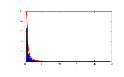
Display the histogram of the samples, along with the probability density function:

>>> import matplotlib.pyplot as plt
>>> import scipy.special as sps
Truncate s values at 50 so plot is interesting
>>> count, bins, ignored = plt.hist(s[s<50], 50, normed=True)
>>> x = np.arange(1., 50.)
>>> y = x**(-a)/sps.zetac(a)
>>> plt.plot(x, y/max(y), linewidth=2, color='r')
>>> plt.show()

(Source code, png, pdf)