scipy.stats.studentized_range#
- scipy.stats.studentized_range = <scipy.stats._continuous_distns.studentized_range_gen object>[source]#
A studentized range continuous random variable.
As an instance of the
rv_continuousclass,studentized_rangeobject inherits from it a collection of generic methods (see below for the full list), and completes them with details specific for this particular distribution.See also
tStudent’s t distribution
Notes
The probability density function for
studentized_rangeis:\[f(x; k, \nu) = \frac{k(k-1)\nu^{\nu/2}}{\Gamma(\nu/2) 2^{\nu/2-1}} \int_{0}^{\infty} \int_{-\infty}^{\infty} s^{\nu} e^{-\nu s^2/2} \phi(z) \phi(sx + z) [\Phi(sx + z) - \Phi(z)]^{k-2} \,dz \,ds\]for \(x ≥ 0\), \(k > 1\), and \(\nu > 0\).
studentized_rangetakeskfor \(k\) anddffor \(\nu\) as shape parameters.When \(\nu\) exceeds 100,000, an asymptotic approximation (infinite degrees of freedom) is used to compute the cumulative distribution function [4].
The probability density above is defined in the “standardized” form. To shift and/or scale the distribution use the
locandscaleparameters. Specifically,studentized_range.pdf(x, k, df, loc, scale)is identically equivalent tostudentized_range.pdf(y, k, df) / scalewithy = (x - loc) / scale. Note that shifting the location of a distribution does not make it a “noncentral” distribution; noncentral generalizations of some distributions are available in separate classes.References
- 1
“Studentized range distribution”, https://en.wikipedia.org/wiki/Studentized_range_distribution
- 2
Batista, Ben Dêivide, et al. “Externally Studentized Normal Midrange Distribution.” Ciência e Agrotecnologia, vol. 41, no. 4, 2017, pp. 378-389., doi:10.1590/1413-70542017414047716.
- 3
Harter, H. Leon. “Tables of Range and Studentized Range.” The Annals of Mathematical Statistics, vol. 31, no. 4, 1960, pp. 1122-1147. JSTOR, www.jstor.org/stable/2237810. Accessed 18 Feb. 2021.
- 4
Lund, R. E., and J. R. Lund. “Algorithm AS 190: Probabilities and Upper Quantiles for the Studentized Range.” Journal of the Royal Statistical Society. Series C (Applied Statistics), vol. 32, no. 2, 1983, pp. 204-210. JSTOR, www.jstor.org/stable/2347300. Accessed 18 Feb. 2021.
Examples
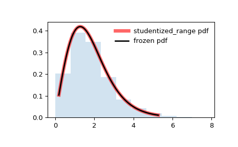
>>> from scipy.stats import studentized_range
>>> import matplotlib.pyplot as plt
>>> fig, ax = plt.subplots(1, 1)
Calculate the first four moments:
>>> k, df = 3, 10
>>> mean, var, skew, kurt = studentized_range.stats(k, df, moments='mvsk')
Display the probability density function (
pdf):>>> x = np.linspace(studentized_range.ppf(0.01, k, df), ... studentized_range.ppf(0.99, k, df), 100) >>> ax.plot(x, studentized_range.pdf(x, k, df), ... 'r-', lw=5, alpha=0.6, label='studentized_range pdf')
Alternatively, the distribution object can be called (as a function) to fix the shape, location and scale parameters. This returns a “frozen” RV object holding the given parameters fixed.
Freeze the distribution and display the frozen
pdf:>>> rv = studentized_range(k, df) >>> ax.plot(x, rv.pdf(x), 'k-', lw=2, label='frozen pdf')
Check accuracy of
cdfandppf:>>> vals = studentized_range.ppf([0.001, 0.5, 0.999], k, df) >>> np.allclose([0.001, 0.5, 0.999], studentized_range.cdf(vals, k, df)) True
Rather than using (
studentized_range.rvs) to generate random variates, which is very slow for this distribution, we can approximate the inverse CDF using an interpolator, and then perform inverse transform sampling with this approximate inverse CDF.This distribution has an infinite but thin right tail, so we focus our attention on the leftmost 99.9 percent.
>>> a, b = studentized_range.ppf([0, .999], k, df)
>>> a, b
0, 7.41058083802274
>>> from scipy.interpolate import interp1d
>>> rng = np.random.default_rng()
>>> xs = np.linspace(a, b, 50)
>>> cdf = studentized_range.cdf(xs, k, df)
# Create an interpolant of the inverse CDF
>>> ppf = interp1d(cdf, xs, fill_value='extrapolate')
# Perform inverse transform sampling using the interpolant
>>> r = ppf(rng.uniform(size=1000))
And compare the histogram:
>>> ax.hist(r, density=True, histtype='stepfilled', alpha=0.2)
>>> ax.legend(loc='best', frameon=False)
>>> plt.show()
Methods
rvs(k, df, loc=0, scale=1, size=1, random_state=None)
Random variates.
pdf(x, k, df, loc=0, scale=1)
Probability density function.
logpdf(x, k, df, loc=0, scale=1)
Log of the probability density function.
cdf(x, k, df, loc=0, scale=1)
Cumulative distribution function.
logcdf(x, k, df, loc=0, scale=1)
Log of the cumulative distribution function.
sf(x, k, df, loc=0, scale=1)
Survival function (also defined as
1 - cdf, but sf is sometimes more accurate).logsf(x, k, df, loc=0, scale=1)
Log of the survival function.
ppf(q, k, df, loc=0, scale=1)
Percent point function (inverse of
cdf— percentiles).isf(q, k, df, loc=0, scale=1)
Inverse survival function (inverse of
sf).moment(n, k, df, loc=0, scale=1)
Non-central moment of order n
stats(k, df, loc=0, scale=1, moments=’mv’)
Mean(‘m’), variance(‘v’), skew(‘s’), and/or kurtosis(‘k’).
entropy(k, df, loc=0, scale=1)
(Differential) entropy of the RV.
fit(data)
Parameter estimates for generic data. See scipy.stats.rv_continuous.fit for detailed documentation of the keyword arguments.
expect(func, args=(k, df), loc=0, scale=1, lb=None, ub=None, conditional=False, **kwds)
Expected value of a function (of one argument) with respect to the distribution.
median(k, df, loc=0, scale=1)
Median of the distribution.
mean(k, df, loc=0, scale=1)
Mean of the distribution.
var(k, df, loc=0, scale=1)
Variance of the distribution.
std(k, df, loc=0, scale=1)
Standard deviation of the distribution.
interval(alpha, k, df, loc=0, scale=1)
Endpoints of the range that contains fraction alpha [0, 1] of the distribution