scipy.stats.sampling.NumericalInversePolynomial

class scipy.stats.sampling.NumericalInversePolynomial(dist, *, mode=None, center=None, domain=None, order=5, u_resolution=1e-10, random_state=None)

Polynomial interpolation based INVersion of CDF (PINV).

PINV is a variant of numerical inversion, where the inverse CDF is approximated using Newton’s interpolating formula. The interval [0,1] is split into several subintervals. In each of these, the inverse CDF is constructed at nodes (CDF(x),x) for some points x in this subinterval. If the PDF is given, then the CDF is computed numerically from the given PDF using adaptive Gauss-Lobatto integration with 5 points. Subintervals are split until the requested accuracy goal is reached.

The method is not exact, as it only produces random variates of the approximated distribution. Nevertheless, the maximal tolerated approximation error can be set to be the resolution (but, of course, is bounded by the machine precision). We use the u-error |U - CDF(X)| to measure the error where X is the approximate percentile corressponding to the quantile U i.e. X = approx_ppf(U). We call the maximal tolerated u-error the u-resolution of the algorithm.

Both the order of the interpolating polynomial and the u-resolution can be selected. Note that very small values of the u-resolution are possible but increase the cost for the setup step.

The interpolating polynomials have to be computed in a setup step. However, it only works for distributions with bounded domain; for distributions with unbounded domain the tails are cut off such that the probability for the tail regions is small compared to the given u-resolution.

The construction of the interpolation polynomial only works when the PDF is unimodal or when the PDF does not vanish between two modes.

There are some restrictions for the given distribution:

• The support of the distribution (i.e., the region where the PDF is strictly positive) must be connected. In practice this means, that the region where PDF is “not too small” must be connected. Unimodal densities satisfy this condition. If this condition is violated then the domain of the distribution might be truncated.

• When the PDF is integrated numerically, then the given PDF must be continuous and should be smooth.

• The PDF must be bounded.

• The algorithm has problems when the distribution has heavy tails (as then the inverse CDF becomes very steep at 0 or 1) and the requested u-resolution is very small. E.g., the Cauchy distribution is likely to show this problem when the requested u-resolution is less then 1.e-12.

Parameters

distobject

An instance of a class with a pdf and optionally a cdf method.

• pdf: PDF of the distribution. The signature of the PDF is expected to be: def pdf(self, x: float) -> float, i.e., the PDF should accept a Python float and return a Python float. It doesn’t need to integrate to 1, i.e., the PDF doesn’t need to be normalized.

• cdf: CDF of the distribution. This method is optional. If provided, it enables the calculation of “u-error”. See u_error. Must have the same signature as the PDF.

modefloat, optional

(Exact) Mode of the distribution. Default is None.

centerfloat, optional

Approximate location of the mode or the mean of the distribution. This location provides some information about the main part of the PDF and is used to avoid numerical problems. Default is None.

domainlist or tuple of length 2, optional

The support of the distribution. Default is None. When None:

• If a support method is provided by the distribution object dist, it is used to set the domain of the distribution.

• Otherwise the support is assumed to be \((-\infty, \infty)\).

orderint, optional

Order of the interpolating polynomial. Valid orders are between 3 and 17. Higher orders result in fewer intervals for the approximations. Default is 5.

u_resolutionfloat, optional

Set maximal tolerated u-error. Values of u_resolution must at least 1.e-15 and 1.e-5 at most. Notice that the resolution of most uniform random number sources is 2-32= 2.3e-10. Thus a value of 1.e-10 leads to an inversion algorithm that could be called exact. For most simulations slightly bigger values for the maximal error are enough as well. Default is 1e-10.

random_state{None, int, numpy.random.Generator,

numpy.random.RandomState}, optional

A NumPy random number generator or seed for the underlying NumPy random number generator used to generate the stream of uniform random numbers. If random_state is None (or np.random), the numpy.random.RandomState singleton is used. If random_state is an int, a new RandomState instance is used, seeded with random_state. If random_state is already a Generator or RandomState instance then that instance is used.

References

1

Derflinger, Gerhard, Wolfgang Hörmann, and Josef Leydold. “Random variate generation by numerical inversion when only the density is known.” ACM Transactions on Modeling and Computer Simulation (TOMACS) 20.4 (2010): 1-25.

2

UNU.RAN reference manual, Section 5.3.12, “PINV – Polynomial interpolation based INVersion of CDF”, https://statmath.wu.ac.at/software/unuran/doc/unuran.html#PINV

Examples

>>> from scipy.stats.sampling import NumericalInversePolynomial
>>> from scipy.stats import norm

To create a generator to sample from the standard normal distribution, do:

>>> class StandardNormal:
...    def pdf(self, x):
...        return np.exp(-0.5 * x*x)
... 
>>> dist = StandardNormal()
>>> urng = np.random.default_rng()
>>> rng = NumericalInversePolynomial(dist, random_state=urng)

Once a generator is created, samples can be drawn from the distribution by calling the rvs method:

>>> rng.rvs()
-1.5244996276336318

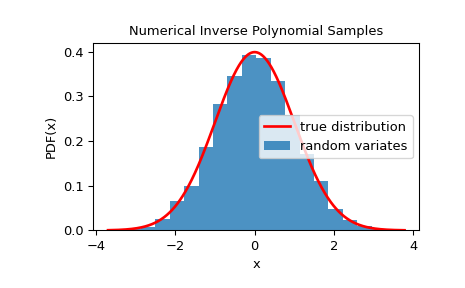
To check that the random variates closely follow the given distribution, we can look at it’s histogram:

>>> import matplotlib.pyplot as plt
>>> rvs = rng.rvs(10000)
>>> x = np.linspace(rvs.min()-0.1, rvs.max()+0.1, 1000)
>>> fx = norm.pdf(x)
>>> plt.plot(x, fx, 'r-', lw=2, label='true distribution')
>>> plt.hist(rvs, bins=20, density=True, alpha=0.8, label='random variates')
>>> plt.xlabel('x')
>>> plt.ylabel('PDF(x)')
>>> plt.title('Numerical Inverse Polynomial Samples')
>>> plt.legend()
>>> plt.show()

It is possible to estimate the u-error of the approximated PPF if the exact CDF is available during setup. To do so, pass a dist object with exact CDF of the distribution during initialization:

>>> from scipy.special import ndtr
>>> class StandardNormal:
...    def pdf(self, x):
...        return np.exp(-0.5 * x*x)
...    def cdf(self, x):
...        return ndtr(x)
... 
>>> dist = StandardNormal()
>>> urng = np.random.default_rng()
>>> rng = NumericalInversePolynomial(dist, random_state=urng)

Now, the u-error can be estimated by calling the u_error method. It runs a Monte-Carlo simulation to estimate the u-error. By default, 100000 samples are used. To change this, you can pass the number of samples as an argument:

>>> rng.u_error(sample_size=1000000)  # uses one million samples
UError(max_error=8.785994154436594e-11, mean_absolute_error=2.930890027826552e-11)

This returns a namedtuple which contains the maximum u-error and the mean absolute u-error.

The u-error can be reduced by decreasing the u-resolution (maximum allowed u-error):

>>> urng = np.random.default_rng()
>>> rng = NumericalInversePolynomial(dist, u_resolution=1.e-12, random_state=urng)
>>> rng.u_error(sample_size=1000000)
UError(max_error=9.07496300328603e-13, mean_absolute_error=3.5255644517257716e-13)

Note that this comes at the cost of increased setup time.

The approximated PPF can be evaluated by calling the ppf method:

>>> rng.ppf(0.975)
1.9599639857012559
>>> norm.ppf(0.975)
1.959963984540054

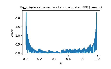
Since the PPF of the normal distribution is available as a special function, we can also check the x-error, i.e. the difference between the approximated PPF and exact PPF:

>>> import matplotlib.pyplot as plt
>>> u = np.linspace(0.01, 0.99, 1000)
>>> approxppf = rng.ppf(u)
>>> exactppf = norm.ppf(u)
>>> error = np.abs(exactppf - approxppf)
>>> plt.plot(u, error)
>>> plt.xlabel('u')
>>> plt.ylabel('error')
>>> plt.title('Error between exact and approximated PPF (x-error)')
>>> plt.show()

Attributes

intervals

Get the number of intervals used in the computation.

Methods

cdf(x)	Approximated cumulative distribution function of the given distribution.
ppf(u)	Approximated PPF of the given distribution.
rvs([size, random_state])	Sample from the distribution.
set_random_state([random_state])	Set the underlying uniform random number generator.
u_error([sample_size])	Estimate the u-error of the approximation using Monte Carlo simulation.

previous

scipy.stats.sampling.NumericalInverseHermite.u_error

next

scipy.stats.sampling.NumericalInversePolynomial.cdf