scipy.stats.norminvgauss#
- scipy.stats.norminvgauss = <scipy.stats._continuous_distns.norminvgauss_gen object>[source]#
A Normal Inverse Gaussian continuous random variable.
As an instance of the
rv_continuousclass,norminvgaussobject inherits from it a collection of generic methods (see below for the full list), and completes them with details specific for this particular distribution.Notes
The probability density function for
norminvgaussis:\[f(x, a, b) = \frac{a \, K_1(a \sqrt{1 + x^2})}{\pi \sqrt{1 + x^2}} \, \exp(\sqrt{a^2 - b^2} + b x)\]where \(x\) is a real number, the parameter \(a\) is the tail heaviness and \(b\) is the asymmetry parameter satisfying \(a > 0\) and \(|b| <= a\). \(K_1\) is the modified Bessel function of second kind (
scipy.special.k1).The probability density above is defined in the “standardized” form. To shift and/or scale the distribution use the
locandscaleparameters. Specifically,norminvgauss.pdf(x, a, b, loc, scale)is identically equivalent tonorminvgauss.pdf(y, a, b) / scalewithy = (x - loc) / scale. Note that shifting the location of a distribution does not make it a “noncentral” distribution; noncentral generalizations of some distributions are available in separate classes.A normal inverse Gaussian random variable Y with parameters a and b can be expressed as a normal mean-variance mixture: Y = b * V + sqrt(V) * X where X is norm(0,1) and V is invgauss(mu=1/sqrt(a**2 - b**2)). This representation is used to generate random variates.
Another common parametrization of the distribution (see Equation 2.1 in [2]) is given by the following expression of the pdf:
\[g(x, \alpha, \beta, \delta, \mu) = \frac{\alpha\delta K_1\left(\alpha\sqrt{\delta^2 + (x - \mu)^2}\right)} {\pi \sqrt{\delta^2 + (x - \mu)^2}} \, e^{\delta \sqrt{\alpha^2 - \beta^2} + \beta (x - \mu)}\]In SciPy, this corresponds to a = alpha * delta, b = beta * delta, loc = mu, scale=delta.
References
- 1
O. Barndorff-Nielsen, “Hyperbolic Distributions and Distributions on Hyperbolae”, Scandinavian Journal of Statistics, Vol. 5(3), pp. 151-157, 1978.
- 2
O. Barndorff-Nielsen, “Normal Inverse Gaussian Distributions and Stochastic Volatility Modelling”, Scandinavian Journal of Statistics, Vol. 24, pp. 1-13, 1997.
Examples
>>> from scipy.stats import norminvgauss
>>> import matplotlib.pyplot as plt
>>> fig, ax = plt.subplots(1, 1)
Calculate the first four moments:
>>> a, b = 1.25, 0.5
>>> mean, var, skew, kurt = norminvgauss.stats(a, b, moments='mvsk')
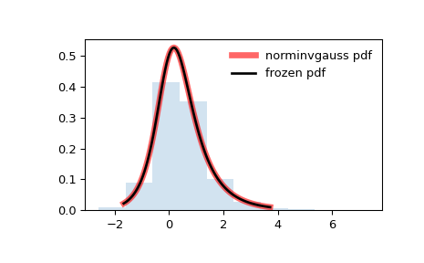
Display the probability density function (
pdf):>>> x = np.linspace(norminvgauss.ppf(0.01, a, b), ... norminvgauss.ppf(0.99, a, b), 100) >>> ax.plot(x, norminvgauss.pdf(x, a, b), ... 'r-', lw=5, alpha=0.6, label='norminvgauss pdf')
Alternatively, the distribution object can be called (as a function) to fix the shape, location and scale parameters. This returns a “frozen” RV object holding the given parameters fixed.
Freeze the distribution and display the frozen
pdf:>>> rv = norminvgauss(a, b) >>> ax.plot(x, rv.pdf(x), 'k-', lw=2, label='frozen pdf')
Check accuracy of
cdfandppf:>>> vals = norminvgauss.ppf([0.001, 0.5, 0.999], a, b) >>> np.allclose([0.001, 0.5, 0.999], norminvgauss.cdf(vals, a, b)) True
Generate random numbers:
>>> r = norminvgauss.rvs(a, b, size=1000)
And compare the histogram:
>>> ax.hist(r, density=True, histtype='stepfilled', alpha=0.2)
>>> ax.legend(loc='best', frameon=False)
>>> plt.show()
Methods
rvs(a, b, loc=0, scale=1, size=1, random_state=None)
Random variates.
pdf(x, a, b, loc=0, scale=1)
Probability density function.
logpdf(x, a, b, loc=0, scale=1)
Log of the probability density function.
cdf(x, a, b, loc=0, scale=1)
Cumulative distribution function.
logcdf(x, a, b, loc=0, scale=1)
Log of the cumulative distribution function.
sf(x, a, b, loc=0, scale=1)
Survival function (also defined as
1 - cdf, but sf is sometimes more accurate).logsf(x, a, b, loc=0, scale=1)
Log of the survival function.
ppf(q, a, b, loc=0, scale=1)
Percent point function (inverse of
cdf— percentiles).isf(q, a, b, loc=0, scale=1)
Inverse survival function (inverse of
sf).moment(n, a, b, loc=0, scale=1)
Non-central moment of order n
stats(a, b, loc=0, scale=1, moments=’mv’)
Mean(‘m’), variance(‘v’), skew(‘s’), and/or kurtosis(‘k’).
entropy(a, b, loc=0, scale=1)
(Differential) entropy of the RV.
fit(data)
Parameter estimates for generic data. See scipy.stats.rv_continuous.fit for detailed documentation of the keyword arguments.
expect(func, args=(a, b), loc=0, scale=1, lb=None, ub=None, conditional=False, **kwds)
Expected value of a function (of one argument) with respect to the distribution.
median(a, b, loc=0, scale=1)
Median of the distribution.
mean(a, b, loc=0, scale=1)
Mean of the distribution.
var(a, b, loc=0, scale=1)
Variance of the distribution.
std(a, b, loc=0, scale=1)
Standard deviation of the distribution.
interval(alpha, a, b, loc=0, scale=1)
Endpoints of the range that contains fraction alpha [0, 1] of the distribution