scipy.signal.zoom_fft#

scipy.signal.zoom_fft(x, fn, m=None, *, fs=2, endpoint=False, axis=- 1)[source]#

Compute the DFT of x only for frequencies in range fn.

Parameters

xarray: The signal to transform.
fnarray_like: A length-2 sequence [f1, f2] giving the frequency range, or a scalar, for which the range [0, fn] is assumed.
mint, optional: The number of points to evaluate. The default is the length of x.
fsfloat, optional: The sampling frequency. If fs=10 represented 10 kHz, for example, then f1 and f2 would also be given in kHz. The default sampling frequency is 2, so f1 and f2 should be in the range [0, 1] to keep the transform below the Nyquist frequency.
endpointbool, optional: If True, f2 is the last sample. Otherwise, it is not included. Default is False.
axisint, optional: Axis over which to compute the FFT. If not given, the last axis is used.

Returns

outndarray: The transformed signal. The Fourier transform will be calculated at the points f1, f1+df, f1+2df, …, f2, where df=(f2-f1)/m.

See also

ZoomFFT: Class that creates a callable partial FFT function.

Notes

The defaults are chosen such that signal.zoom_fft(x, 2) is equivalent to fft.fft(x) and, if m > len(x), that signal.zoom_fft(x, 2, m) is equivalent to fft.fft(x, m).

To graph the magnitude of the resulting transform, use:

plot(linspace(f1, f2, m, endpoint=False), abs(zoom_fft(x, [f1, f2], m)))

If the transform needs to be repeated, use ZoomFFT to construct a specialized transform function which can be reused without recomputing constants.

Examples

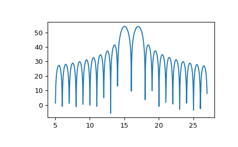
To plot the transform results use something like the following:

>>> from scipy.signal import zoom_fft
>>> t = np.linspace(0, 1, 1021)
>>> x = np.cos(2*np.pi*15*t) + np.sin(2*np.pi*17*t)
>>> f1, f2 = 5, 27
>>> X = zoom_fft(x, [f1, f2], len(x), fs=1021)
>>> f = np.linspace(f1, f2, len(x))
>>> import matplotlib.pyplot as plt
>>> plt.plot(f, 20*np.log10(np.abs(X)))
>>> plt.show()

../../_images/scipy-signal-zoom_fft-1.png

scipy.signal.czt

scipy.signal.CZT