scipy.signal.bilinear_zpk#
- scipy.signal.bilinear_zpk(z, p, k, fs)[source]#
Return a digital IIR filter from an analog one using a bilinear transform.
Transform a set of poles and zeros from the analog s-plane to the digital z-plane using Tustin’s method, which substitutes
(z-1) / (z+1)fors, maintaining the shape of the frequency response.- Parameters
- zarray_like
Zeros of the analog filter transfer function.
- parray_like
Poles of the analog filter transfer function.
- kfloat
System gain of the analog filter transfer function.
- fsfloat
Sample rate, as ordinary frequency (e.g., hertz). No prewarping is done in this function.
- Returns
- zndarray
Zeros of the transformed digital filter transfer function.
- pndarray
Poles of the transformed digital filter transfer function.
- kfloat
System gain of the transformed digital filter.
Notes
New in version 1.1.0.
Examples
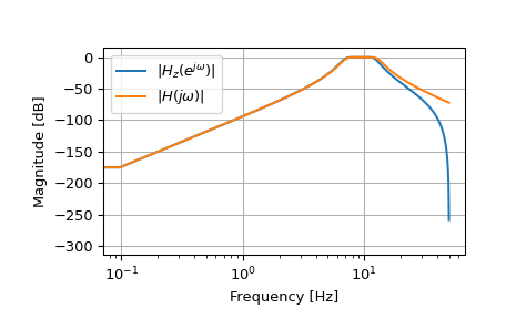
>>> from scipy import signal
>>> import matplotlib.pyplot as plt
>>> fs = 100
>>> bf = 2 * np.pi * np.array([7, 13])
>>> filts = signal.lti(*signal.butter(4, bf, btype='bandpass', analog=True,
...                                   output='zpk'))
>>> filtz = signal.lti(*signal.bilinear_zpk(filts.zeros, filts.poles,
...                                         filts.gain, fs))
>>> wz, hz = signal.freqz_zpk(filtz.zeros, filtz.poles, filtz.gain)
>>> ws, hs = signal.freqs_zpk(filts.zeros, filts.poles, filts.gain,
...                           worN=fs*wz)
>>> plt.semilogx(wz*fs/(2*np.pi), 20*np.log10(np.abs(hz).clip(1e-15)),
...              label=r'$|H_z(e^{j \omega})|$')
>>> plt.semilogx(wz*fs/(2*np.pi), 20*np.log10(np.abs(hs).clip(1e-15)),
...              label=r'$|H(j \omega)|$')
>>> plt.legend()
>>> plt.xlabel('Frequency [Hz]')
>>> plt.ylabel('Magnitude [dB]')
>>> plt.grid()