scipy.fft.fftn#

scipy.fft.fftn(x, s=None, axes=None, norm=None, overwrite_x=False, workers=None, *, plan=None)[source]#

Compute the N-D discrete Fourier Transform.

This function computes the N-D discrete Fourier Transform over any number of axes in an M-D array by means of the Fast Fourier Transform (FFT).

Parameters

xarray_like: Input array, can be complex.
ssequence of ints, optional: Shape (length of each transformed axis) of the output (s[0] refers to axis 0, s[1] to axis 1, etc.). This corresponds to n for fft(x, n). Along any axis, if the given shape is smaller than that of the input, the input is cropped. If it is larger, the input is padded with zeros. if s is not given, the shape of the input along the axes specified by axes is used.
axessequence of ints, optional: Axes over which to compute the FFT. If not given, the last len(s) axes are used, or all axes if s is also not specified.
norm{“backward”, “ortho”, “forward”}, optional: Normalization mode (see fft). Default is “backward”.
overwrite_xbool, optional: If True, the contents of x can be destroyed; the default is False. See fft for more details.
workersint, optional: Maximum number of workers to use for parallel computation. If negative, the value wraps around from os.cpu_count(). See fft for more details.
planobject, optional: This argument is reserved for passing in a precomputed plan provided by downstream FFT vendors. It is currently not used in SciPy.

New in version 1.5.0.

Returns

outcomplex ndarray: The truncated or zero-padded input, transformed along the axes indicated by axes, or by a combination of s and x, as explained in the parameters section above.

Raises

ValueError: If s and axes have different length.
IndexError: If an element of axes is larger than than the number of axes of x.

See also

ifftn: The inverse of fftn, the inverse N-D FFT.
fft: The 1-D FFT, with definitions and conventions used.
rfftn: The N-D FFT of real input.
fft2: The 2-D FFT.
fftshift: Shifts zero-frequency terms to centre of array.

Notes

The output, analogously to fft, contains the term for zero frequency in the low-order corner of all axes, the positive frequency terms in the first half of all axes, the term for the Nyquist frequency in the middle of all axes and the negative frequency terms in the second half of all axes, in order of decreasingly negative frequency.

Examples

>>> import scipy.fft
>>> x = np.mgrid[:3, :3, :3][0]
>>> scipy.fft.fftn(x, axes=(1, 2))
array([[[ 0.+0.j,   0.+0.j,   0.+0.j], # may vary
        [ 0.+0.j,   0.+0.j,   0.+0.j],
        [ 0.+0.j,   0.+0.j,   0.+0.j]],
       [[ 9.+0.j,   0.+0.j,   0.+0.j],
        [ 0.+0.j,   0.+0.j,   0.+0.j],
        [ 0.+0.j,   0.+0.j,   0.+0.j]],
       [[18.+0.j,   0.+0.j,   0.+0.j],
        [ 0.+0.j,   0.+0.j,   0.+0.j],
        [ 0.+0.j,   0.+0.j,   0.+0.j]]])
>>> scipy.fft.fftn(x, (2, 2), axes=(0, 1))
array([[[ 2.+0.j,  2.+0.j,  2.+0.j], # may vary
        [ 0.+0.j,  0.+0.j,  0.+0.j]],
       [[-2.+0.j, -2.+0.j, -2.+0.j],
        [ 0.+0.j,  0.+0.j,  0.+0.j]]])

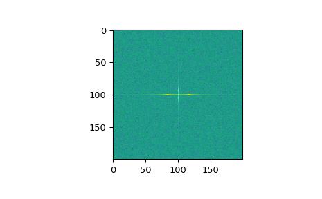
>>> import matplotlib.pyplot as plt
>>> rng = np.random.default_rng()
>>> [X, Y] = np.meshgrid(2 * np.pi * np.arange(200) / 12,
...                      2 * np.pi * np.arange(200) / 34)
>>> S = np.sin(X) + np.cos(Y) + rng.uniform(0, 1, X.shape)
>>> FS = scipy.fft.fftn(S)
>>> plt.imshow(np.log(np.abs(scipy.fft.fftshift(FS))**2))
<matplotlib.image.AxesImage object at 0x...>
>>> plt.show()

scipy.fft.ifft2

scipy.fft.ifftn