scipy.signal.morlet#

scipy.signal.morlet(M, w=5.0, s=1.0, complete=True)[source]#

Complex Morlet wavelet.

Parameters:

Mint: Length of the wavelet.
wfloat, optional: Omega0. Default is 5
sfloat, optional: Scaling factor, windowed from -s*2*pi to +s*2*pi. Default is 1.
completebool, optional: Whether to use the complete or the standard version.

Returns:

morlet(M,) ndarray

See also

morlet2: Implementation of Morlet wavelet, compatible with cwt.
scipy.signal.gausspulse

Notes

The standard version:

pi**-0.25 * exp(1j*w*x) * exp(-0.5*(x**2))

This commonly used wavelet is often referred to simply as the Morlet wavelet. Note that this simplified version can cause admissibility problems at low values of w.

The complete version:

pi**-0.25 * (exp(1j*w*x) - exp(-0.5*(w**2))) * exp(-0.5*(x**2))

This version has a correction term to improve admissibility. For w greater than 5, the correction term is negligible.

Note that the energy of the return wavelet is not normalised according to s.

The fundamental frequency of this wavelet in Hz is given by f = 2*s*w*r / M where r is the sampling rate.

Note: This function was created before cwt and is not compatible with it.

Examples

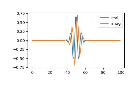
>>> from scipy import signal
>>> import matplotlib.pyplot as plt

>>> M = 100
>>> s = 4.0
>>> w = 2.0
>>> wavelet = signal.morlet(M, s, w)
>>> plt.plot(wavelet.real, label="real")
>>> plt.plot(wavelet.imag, label="imag")
>>> plt.legend()
>>> plt.show()