Interpolate transition guide

This notebook contains three sets of demonstrations:

• lower-level FITPACK replacements for scipy.interpolate.interp2d for legacy bug-for-bug compatible scipy.interpolate.interp2d replacements;

• recommended replacements for scipy.interpolate.interp2d for use in new code;

• a demonstration of failure modes of 2D FITPACK-based linear interpolation and recommended replacements.

Note: Since this notebook shows usage of interp2d (which is marked for deprecation), we will silence deprecation warnings for simplicity:

import warnings
warnings.filterwarnings('ignore')

1. How to transition away from using interp2d

interp2d silently switches between interpolation on a 2D regular grid and interpolatin 2D scattered data. The switch is based on the lengths of the (raveled) x, y, and z arrays. In short, for regular grid use scipy.interpolate.RectBivariateSpline; for scattered interpolation, use the bisprep/bisplev combo. Below we give examples of the literal point-for-point transition, which should preserve the interp2d results exactly.

1.1 interp2d on a regular grid

We start from the (slightly modified) docstring example.

import numpy as np
import matplotlib.pyplot as plt
from scipy.interpolate import interp2d, RectBivariateSpline

x = np.arange(-5.01, 5.01, 0.25)
y = np.arange(-5.01, 7.51, 0.25)
xx, yy = np.meshgrid(x, y)
z = np.sin(xx**2 + 2.*yy**2)
f = interp2d(x, y, z, kind='cubic')

This is the “regular grid” code path, because

z.size == len(x) * len(y)

True

Also, note that x.size != y.size:

x.size, y.size

(41, 51)

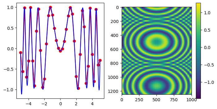
Now, let’s build a convenience function to construct the interpolator and plot it.

def plot(f, xnew, ynew):
    fig, (ax1, ax2) = plt.subplots(1, 2, figsize=(8, 4))
    znew = f(xnew, ynew)

    ax1.plot(x, z[0, :], 'ro-', xnew, znew[0, :], 'b-')

    im = ax2.imshow(znew)
    plt.colorbar(im, ax=ax2)

    plt.show()
    return znew

Plotting:

xnew = np.arange(-5.01, 5.01, 1e-2)
ynew = np.arange(-5.01, 7.51, 1e-2)
znew_i = plot(f, xnew, ynew)

Replacement: Use RectBivariateSpline, the result is identical

Note the transposes: first, in the constructor, second, you need to transpose the result of the evaluation. This is to undo the transposes interp2d does.

r = RectBivariateSpline(x, y, z.T)

rt = lambda xnew, ynew: r(xnew, ynew).T
znew_r = plot(rt, xnew, ynew)

from numpy.testing import assert_allclose
assert_allclose(znew_i, znew_r, atol=1e-14)

1.2. interp2d with full coordinates of points (scattered interpolation)

Here, we flatten the meshgrid from the previous exercise to illustrate the functionality.

xxr = xx.ravel()
yyr = yy.ravel()
zzr = z.ravel()

f = interp2d(xxr, yyr, zzr, kind='cubic')

Note that this the “not regular grid” code path, meant for scattered data, with len(x) == len(y) == len(z).

len(xxr) == len(yyr) == len(zzr)

True

xnew = np.arange(-5.01, 5.01, 1e-2)
ynew = np.arange(-5.01, 7.51, 1e-2)
znew_i = plot(f, xnew, ynew)

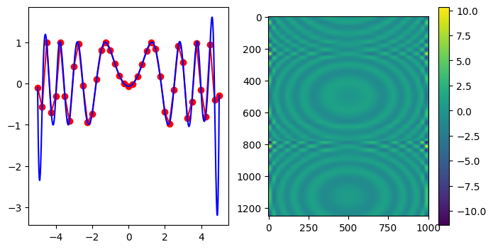
Replacement: Use scipy.interpolate.bisplrep / scipy.interpolate.bisplev directly

from scipy.interpolate import bisplrep, bisplev
tck = bisplrep(xxr, yyr, zzr, kx=3, ky=3, s=0)
# convenience: make up a callable from bisplev
ff = lambda xnew, ynew: bisplev(xnew, ynew, tck).T   # Note the transpose, to mimic what interp2d does

znew_b = plot(ff, xnew, ynew)

assert_allclose(znew_i, znew_b, atol=1e-15)

2. Alternative to interp2d: regular grid

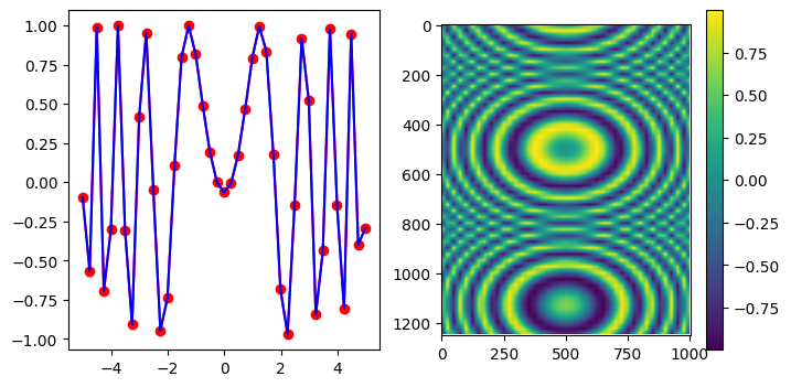
For new code, the recommended alternative is RegularGridInterpolator. It is an independent implementation, not based on FITPACK. Supports nearest, linear interpolation and odd-order tensor product splines.

The spline knots are guaranteed to coincide with the data points.

Note that, here:

1. the tuple argument, is (x, y)

2. z array needs a transpose

3. the keyword name is method, not kind

4. bounds_error argument is True by default.

from scipy.interpolate import RegularGridInterpolator as RGI

r = RGI((x, y), z.T, method='linear', bounds_error=False)

Evaluation: create a 2D meshgrid. Use indexing=’ij’ and sparse=True to save some memory:

xxnew, yynew = np.meshgrid(xnew, ynew, indexing='ij', sparse=True)

Evaluate, note the tuple argument:

znew_reggrid = r((xxnew, yynew))

fig, (ax1, ax2) = plt.subplots(1, 2, figsize=(8, 4))

# Again, note the transpose to undo the `interp2d` convention
znew_reggrid_t = znew_reggrid.T

ax1.plot(x, z[0, :], 'ro-', xnew, znew_reggrid_t[0, :], 'b-')

im = ax2.imshow(znew_reggrid_t)
plt.colorbar(im, ax=ax2)

<matplotlib.colorbar.Colorbar at 0x7f0ecbe021f0>

3. Scattered 2D linear interpolation: prefer LinearNDInterpolator to SmoothBivariateSpline or bisplrep

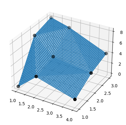
For 2D scattered linear interpolation, both SmoothBivariateSpline and biplrep may either emit warnings, or fail to interpolate the data, or produce splines which with knots away from the data points. “Instead, prefer LinearNDInterpolator, which is based on triangulating the data via QHull.

# TestSmoothBivariateSpline::test_integral
from scipy.interpolate import SmoothBivariateSpline, LinearNDInterpolator

x = np.array([1,1,1,2,2,2,4,4,4])
y = np.array([1,2,3,1,2,3,1,2,3])
z = np.array([0,7,8,3,4,7,1,3,4])

Now, use the linear interpolation over Qhull-based triangulation of data:

xy = np.c_[x, y]   # or just list(zip(x, y))
lut2 = LinearNDInterpolator(xy, z)

X = np.linspace(min(x), max(x))
Y = np.linspace(min(y), max(y))
X, Y = np.meshgrid(X, Y)

The result is easy to understand and interpret:

fig = plt.figure()
ax = fig.add_subplot(projection='3d')

ax.plot_wireframe(X, Y, lut2(X, Y))
ax.scatter(x, y, z,  'o', color='k', s=48)

<mpl_toolkits.mplot3d.art3d.Path3DCollection at 0x7f0ecbd019a0>

Note that bisplrep does something different! It may place spline knots outside of the data.

For illustration, consider the same data from the previous example:

tck = bisplrep(x, y, z, kx=1, ky=1, s=0)

fig = plt.figure()
ax = fig.add_subplot(projection='3d')

xx = np.linspace(min(x), max(x))
yy = np.linspace(min(y), max(y))
X, Y = np.meshgrid(xx, yy)
Z = bisplev(xx, yy, tck)
Z = Z.reshape(*X.shape).T

ax.plot_wireframe(X, Y, Z, rstride=2, cstride=2)
ax.scatter(x, y, z,  'o', color='k', s=48)

<mpl_toolkits.mplot3d.art3d.Path3DCollection at 0x7f0ec82eeac0>

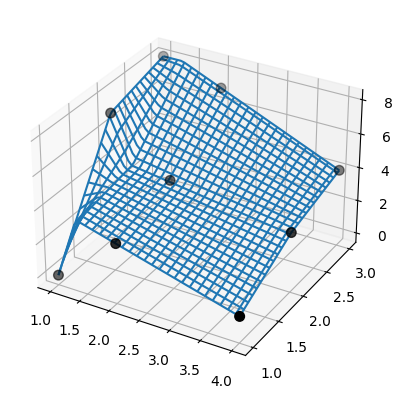
Also, SmoothBivariateSpline fails to interpolate the data. Again, use the same data from the previous example.

lut = SmoothBivariateSpline(x, y, z, kx=1, ky=1, s=0)

fig = plt.figure()
ax = fig.add_subplot(projection='3d')

xx = np.linspace(min(x), max(x))
yy = np.linspace(min(y), max(y))
X, Y = np.meshgrid(xx, yy)

ax.plot_wireframe(X, Y, lut(xx, yy).T, rstride=4, cstride=4)
ax.scatter(x, y, z,  'o', color='k', s=48)

<mpl_toolkits.mplot3d.art3d.Path3DCollection at 0x7f0ec82443d0>

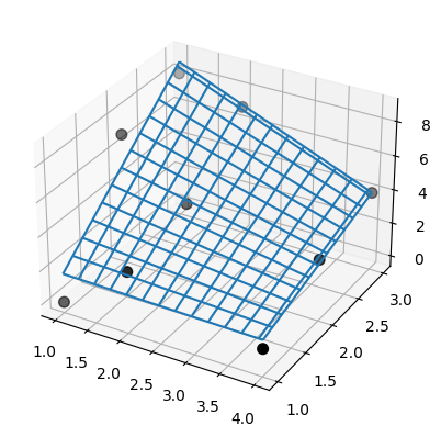
Note that both SmoothBivariateSpline and bisplrep results have artifacts, unlike the LinearNDInterpolator’s. Issues illustrated here were reported for linear interpolation, however the FITPACK knot-selection mechanism does not guarantee to avoid either of these issues for higher-order (e.g. cubic) spline surfaces.