scipy.stats.monte_carlo_test

scipy.stats.monte_carlo_test(sample, rvs, statistic, *, vectorized=None, n_resamples=9999, batch=None, alternative='two-sided', axis=0)

Monte Carlo test that a sample is drawn from a given distribution.

The null hypothesis is that the provided sample was drawn at random from the distribution for which rvs generates random variates. The value of the statistic for the given sample is compared against a Monte Carlo null distribution: the value of the statistic for each of n_resamples samples generated by rvs. This gives the p-value, the probability of observing such an extreme value of the test statistic under the null hypothesis.

Parameters:

samplearray-like

An array of observations.

rvscallable

Generates random variates from the distribution against which sample will be tested. rvs must be a callable that accepts keyword argument size (e.g. rvs(size=(m, n))) and returns an N-d array sample of that shape.

statisticcallable

Statistic for which the p-value of the hypothesis test is to be calculated. statistic must be a callable that accepts a sample (e.g. statistic(sample)) and returns the resulting statistic. If vectorized is set True, statistic must also accept a keyword argument axis and be vectorized to compute the statistic along the provided axis of the sample array.

vectorizedbool, optional

If vectorized is set False, statistic will not be passed keyword argument axis and is expected to calculate the statistic only for 1D samples. If True, statistic will be passed keyword argument axis and is expected to calculate the statistic along axis when passed an ND sample array. If None (default), vectorized will be set True if axis is a parameter of statistic. Use of a vectorized statistic typically reduces computation time.

n_resamplesint, default: 9999

Number of random permutations used to approximate the Monte Carlo null distribution.

batchint, optional

The number of permutations to process in each call to statistic. Memory usage is O(batch`*``sample.size[axis]`). Default is None, in which case batch equals n_resamples.

alternative{‘two-sided’, ‘less’, ‘greater’}

The alternative hypothesis for which the p-value is calculated. For each alternative, the p-value is defined as follows.

• 'greater' : the percentage of the null distribution that is greater than or equal to the observed value of the test statistic.

• 'less' : the percentage of the null distribution that is less than or equal to the observed value of the test statistic.

• 'two-sided' : twice the smaller of the p-values above.

axisint, default: 0

The axis of sample over which to calculate the statistic.

Returns:

statisticfloat or ndarray

The observed test statistic of the sample.

pvaluefloat or ndarray

The p-value for the given alternative.

null_distributionndarray

The values of the test statistic generated under the null hypothesis.

References

[1]

B. Phipson and G. K. Smyth. “Permutation P-values Should Never Be Zero: Calculating Exact P-values When Permutations Are Randomly Drawn.” Statistical Applications in Genetics and Molecular Biology 9.1 (2010).

Examples

Suppose we wish to test whether a small sample has been drawn from a normal distribution. We decide that we will use the skew of the sample as a test statistic, and we will consider a p-value of 0.05 to be statistically significant.

>>> import numpy as np
>>> from scipy import stats
>>> def statistic(x, axis):
...     return stats.skew(x, axis)

After collecting our data, we calculate the observed value of the test statistic.

>>> rng = np.random.default_rng()
>>> x = stats.skewnorm.rvs(a=1, size=50, random_state=rng)
>>> statistic(x, axis=0)
0.12457412450240658

To determine the probability of observing such an extreme value of the skewness by chance if the sample were drawn from the normal distribution, we can perform a Monte Carlo hypothesis test. The test will draw many samples at random from their normal distribution, calculate the skewness of each sample, and compare our original skewness against this distribution to determine an approximate p-value.

>>> from scipy.stats import monte_carlo_test
>>> # because our statistic is vectorized, we pass `vectorized=True`
>>> rvs = lambda size: stats.norm.rvs(size=size, random_state=rng)
>>> res = monte_carlo_test(x, rvs, statistic, vectorized=True)
>>> print(res.statistic)
0.12457412450240658
>>> print(res.pvalue)
0.7012

The probability of obtaining a test statistic less than or equal to the observed value under the null hypothesis is ~70%. This is greater than our chosen threshold of 5%, so we cannot consider this to be significant evidence against the null hypothesis.

Note that this p-value essentially matches that of scipy.stats.skewtest, which relies on an asymptotic distribution of a test statistic based on the sample skewness.

>>> stats.skewtest(x).pvalue
0.6892046027110614

This asymptotic approximation is not valid for small sample sizes, but monte_carlo_test can be used with samples of any size.

>>> x = stats.skewnorm.rvs(a=1, size=7, random_state=rng)
>>> # stats.skewtest(x) would produce an error due to small sample
>>> res = monte_carlo_test(x, rvs, statistic, vectorized=True)

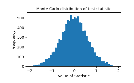
The Monte Carlo distribution of the test statistic is provided for further investigation.

>>> import matplotlib.pyplot as plt
>>> fig, ax = plt.subplots()
>>> ax.hist(res.null_distribution, bins=50)
>>> ax.set_title("Monte Carlo distribution of test statistic")
>>> ax.set_xlabel("Value of Statistic")
>>> ax.set_ylabel("Frequency")
>>> plt.show()