scipy.special.kve

scipy.special.kve(v, z, out=None) = <ufunc 'kve'>

Exponentially scaled modified Bessel function of the second kind.

Returns the exponentially scaled, modified Bessel function of the second kind (sometimes called the third kind) for real order v at complex z:

kve(v, z) = kv(v, z) * exp(z)

Parameters:

varray_like of float

Order of Bessel functions

zarray_like of complex

Argument at which to evaluate the Bessel functions

outndarray, optional

Optional output array for the function results

Returns:

scalar or ndarray

The exponentially scaled modified Bessel function of the second kind.

See also

kv

This function without exponential scaling.

k0e

Faster version of this function for order 0.

k1e

Faster version of this function for order 1.

Notes

Wrapper for AMOS [1] routine zbesk. For a discussion of the algorithm used, see [2] and the references therein.

References

[1]

Donald E. Amos, “AMOS, A Portable Package for Bessel Functions of a Complex Argument and Nonnegative Order”, http://netlib.org/amos/

[2]

Donald E. Amos, “Algorithm 644: A portable package for Bessel functions of a complex argument and nonnegative order”, ACM TOMS Vol. 12 Issue 3, Sept. 1986, p. 265

Examples

Evaluate the function of order 0 at one point.

>>> import numpy as np
>>> from scipy.special import kv, kve
>>> import matplotlib.pyplot as plt
>>> kve(0, 1.)
1.1444630798068949

Evaluate the function at one point for different orders by providing a list or NumPy array as argument for the v parameter:

>>> kve([0, 1, 1.5], 1.)
array([1.14446308, 1.63615349, 2.50662827])

Evaluate the function at several points for order 0 by providing an array for z.

>>> points = np.array([1., 3., 10.])
>>> kve(0, points)
array([1.14446308, 0.6977616 , 0.39163193])

Evaluate the function at several points for different orders by providing arrays for both v for z. Both arrays have to be broadcastable to the correct shape. To calculate the orders 0, 1 and 2 for a 1D array of points:

>>> kve([[0], [1], [2]], points)
array([[1.14446308, 0.6977616 , 0.39163193],
       [1.63615349, 0.80656348, 0.41076657],
       [4.41677005, 1.23547058, 0.47378525]])

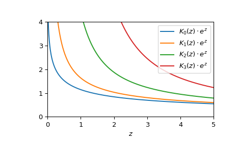
Plot the functions of order 0 to 3 from 0 to 5.

>>> fig, ax = plt.subplots()
>>> x = np.linspace(0., 5., 1000)
>>> for i in range(4):
...     ax.plot(x, kve(i, x), label=f'$K_{i!r}(z)\cdot e^z$')
>>> ax.legend()
>>> ax.set_xlabel(r"$z$")
>>> ax.set_ylim(0, 4)
>>> ax.set_xlim(0, 5)
>>> plt.show()

Exponentially scaled Bessel functions are useful for large arguments for which the unscaled Bessel functions over- or underflow. In the following example kv returns 0 whereas kve still returns a useful finite number.

>>> kv(3, 1000.), kve(3, 1000.)
(0.0, 0.03980696128440973)