Signal Processing (scipy.signal)
The signal processing toolbox currently contains some filtering functions, a limited set of filter design tools, and a few B-spline interpolation algorithms for one- and two-dimensional data. While the B-spline algorithms could technically be placed under the interpolation category, they are included here because they only work with equally-spaced data and make heavy use of filter-theory and transfer-function formalism to provide a fast B-spline transform. To understand this section you will need to understand that a signal in SciPy is an array of real or complex numbers.
B-splines
A B-spline is an approximation of a continuous function over a finite-
domain in terms of B-spline coefficients and knot points. If the knot-
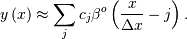
points are equally spaced with spacing  , then the B-spline
approximation to a 1-dimensional function is the finite-basis expansion.
, then the B-spline
approximation to a 1-dimensional function is the finite-basis expansion.
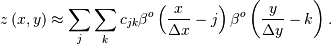
In two dimensions with knot-spacing and  , the
function representation is
, the
function representation is
In these expressions,  is the space-limited
B-spline basis function of order,
is the space-limited
B-spline basis function of order,  . The requirement of equally-spaced
knot-points and equally-spaced data points, allows the development of fast
(inverse-filtering) algorithms for determining the coefficients,
. The requirement of equally-spaced
knot-points and equally-spaced data points, allows the development of fast
(inverse-filtering) algorithms for determining the coefficients,  , from sample-values,
  . Unlike the general spline interpolation
algorithms, these algorithms can quickly find the spline coefficients for large
images.
. Unlike the general spline interpolation
algorithms, these algorithms can quickly find the spline coefficients for large
images.
The advantage of representing a set of samples via B-spline basis functions is that continuous-domain operators (derivatives, re- sampling, integral, etc.) which assume that the data samples are drawn from an underlying continuous function can be computed with relative ease from the spline coefficients. For example, the second-derivative of a spline is
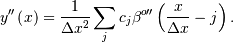
Using the property of B-splines that
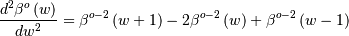
it can be seen that
![y^{\prime\prime}\left(x\right)=\frac{1}{\Delta x^{2}}\sum_{j}c_{j}\left[\beta^{o-2}\left(\frac{x}{\Delta x}-j+1\right)-2\beta^{o-2}\left(\frac{x}{\Delta x}-j\right)+\beta^{o-2}\left(\frac{x}{\Delta x}-j-1\right)\right].](../_images/math/e50d559ebe3fdc3ff7bec7cac8e18230d8b7c943.png)
If  , then at the sample points,
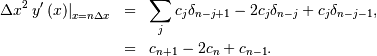
Thus, the second-derivative signal can be easily calculated from the spline fit. if desired, smoothing splines can be found to make the second-derivative less sensitive to random-errors.
The savvy reader will have already noticed that the data samples are related to the knot coefficients via a convolution operator, so that simple convolution with the sampled B-spline function recovers the original data from the spline coefficients. The output of convolutions can change depending on how boundaries are handled (this becomes increasingly more important as the number of dimensions in the data- set increases). The algorithms relating to B-splines in the signal- processing sub package assume mirror-symmetric boundary conditions. Thus, spline coefficients are computed based on that assumption, and data-samples can be recovered exactly from the spline coefficients by assuming them to be mirror-symmetric also.
Currently the package provides functions for determining second- and third-
order cubic spline coefficients from equally spaced samples in one- and two-
dimensions (qspline1d, qspline2d, cspline1d,
cspline2d). The package also supplies a function ( bspline )
for evaluating the bspline basis function,  for
arbitrary order and
for
arbitrary order and  For large , the B-spline basis
function can be approximated well by a zero-mean Gaussian function with
standard-deviation equal to
For large , the B-spline basis
function can be approximated well by a zero-mean Gaussian function with
standard-deviation equal to  :
:
A function to compute this Gaussian for arbitrary  and is
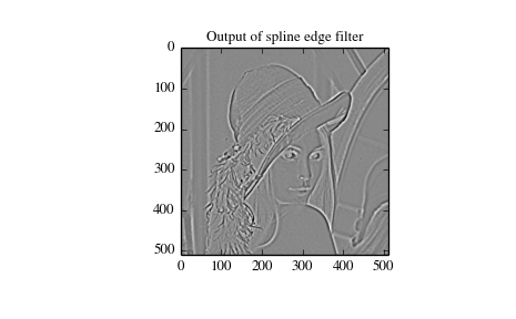
also available ( gauss_spline ). The following code and Figure uses
spline-filtering to compute an edge-image (the second-derivative of a smoothed
spline) of Lena’s face which is an array returned by the command misc.lena.
The command sepfir2d was used to apply a separable two-dimensional FIR
filter with mirror- symmetric boundary conditions to the spline coefficients.
This function is ideally suited for reconstructing samples from spline
coefficients and is faster than convolve2d which convolves arbitrary
two-dimensional filters and allows for choosing mirror-symmetric boundary
conditions.
and is
also available ( gauss_spline ). The following code and Figure uses
spline-filtering to compute an edge-image (the second-derivative of a smoothed
spline) of Lena’s face which is an array returned by the command misc.lena.
The command sepfir2d was used to apply a separable two-dimensional FIR
filter with mirror- symmetric boundary conditions to the spline coefficients.
This function is ideally suited for reconstructing samples from spline
coefficients and is faster than convolve2d which convolves arbitrary
two-dimensional filters and allows for choosing mirror-symmetric boundary
conditions.
>>> from numpy import *
>>> from scipy import signal, misc
>>> import matplotlib.pyplot as plt
>>> image = misc.lena().astype(float32)
>>> derfilt = array([1.0,-2,1.0],float32)
>>> ck = signal.cspline2d(image,8.0)
>>> deriv = signal.sepfir2d(ck, derfilt, [1]) + \
>>>         signal.sepfir2d(ck, [1], derfilt)
Alternatively we could have done:
laplacian = array([[0,1,0],[1,-4,1],[0,1,0]],float32)
deriv2 = signal.convolve2d(ck,laplacian,mode='same',boundary='symm')
>>> plt.figure()
>>> plt.imshow(image)
>>> plt.gray()
>>> plt.title('Original image')
>>> plt.show()

>>> plt.figure()
>>> plt.imshow(deriv)
>>> plt.gray()
>>> plt.title('Output of spline edge filter')
>>> plt.show()
Filtering
Filtering is a generic name for any system that modifies an input
signal in some way. In SciPy a signal can be thought of as a Numpy
array. There are different kinds of filters for different kinds of
operations. There are two broad kinds of filtering operations: linear
and non-linear. Linear filters can always be reduced to multiplication
of the flattened Numpy array by an appropriate matrix resulting in
another flattened Numpy array. Of course, this is not usually the best
way to compute the filter as the matrices and vectors involved may be
huge. For example filtering a  image with this
method would require multiplication of a
image with this
method would require multiplication of a  matrix with a
  vector. Just trying to store the
matrix using a standard Numpy array would
require
vector. Just trying to store the
matrix using a standard Numpy array would
require  elements. At 4 bytes per element this
would require
elements. At 4 bytes per element this
would require  of memory. In most applications
most of the elements of this matrix are zero and a different method
for computing the output of the filter is employed.
of memory. In most applications
most of the elements of this matrix are zero and a different method
for computing the output of the filter is employed.
Convolution/Correlation
Many linear filters also have the property of shift-invariance. This means that the filtering operation is the same at different locations in the signal and it implies that the filtering matrix can be constructed from knowledge of one row (or column) of the matrix alone. In this case, the matrix multiplication can be accomplished using Fourier transforms.
Let ![x\left[n\right]](../_images/math/623877151151bf1c15e9891b03ef2cd36091dd2d.png) define a one-dimensional signal indexed by the
integer
define a one-dimensional signal indexed by the
integer  Full convolution of two one-dimensional signals can be
expressed as
Full convolution of two one-dimensional signals can be
expressed as
![y\left[n\right]=\sum_{k=-\infty}^{\infty}x\left[k\right]h\left[n-k\right].](../_images/math/8c8996a7fc97feff5bd1aa524984d2325502e2a5.png)
This equation can only be implemented directly if we limit the
sequences to finite support sequences that can be stored in a
computer, choose  to be the starting point of both
sequences, let
to be the starting point of both
sequences, let  be that value for which
![y\left[n\right]=0](../_images/math/9ae23804358b4f1a3c3adca008a4a33e2e488466.png) for all
for all  and
and  be
that value for which
be
that value for which ![x\left[n\right]=0](../_images/math/3503a06b2728bcfdb559fb2a045423027b292cb2.png) for all
for all  ,
then the discrete convolution expression is
,
then the discrete convolution expression is
![y\left[n\right]=\sum_{k=\max\left(n-M,0\right)}^{\min\left(n,K\right)}x\left[k\right]h\left[n-k\right].](../_images/math/1281669435546d9b2a732b3c00be0a95c1a4a394.png)
For convenience assume  Then, more explicitly the output of
this operation is
Then, more explicitly the output of
this operation is
![\begin{eqnarray*} y\left[0\right] & = & x\left[0\right]h\left[0\right]\\ y\left[1\right] & = & x\left[0\right]h\left[1\right]+x\left[1\right]h\left[0\right]\\ y\left[2\right] & = & x\left[0\right]h\left[2\right]+x\left[1\right]h\left[1\right]+x\left[2\right]h\left[0\right]\\ \vdots & \vdots & \vdots\\ y\left[M\right] & = & x\left[0\right]h\left[M\right]+x\left[1\right]h\left[M-1\right]+\cdots+x\left[M\right]h\left[0\right]\\ y\left[M+1\right] & = & x\left[1\right]h\left[M\right]+x\left[2\right]h\left[M-1\right]+\cdots+x\left[M+1\right]h\left[0\right]\\ \vdots & \vdots & \vdots\\ y\left[K\right] & = & x\left[K-M\right]h\left[M\right]+\cdots+x\left[K\right]h\left[0\right]\\ y\left[K+1\right] & = & x\left[K+1-M\right]h\left[M\right]+\cdots+x\left[K\right]h\left[1\right]\\ \vdots & \vdots & \vdots\\ y\left[K+M-1\right] & = & x\left[K-1\right]h\left[M\right]+x\left[K\right]h\left[M-1\right]\\ y\left[K+M\right] & = & x\left[K\right]h\left[M\right].\end{eqnarray*}](../_images/math/747737401b5adab02c12c96658b539922ef31c3f.png)
Thus, the full discrete convolution of two finite sequences of lengths
and respectively results in a finite sequence of length

One dimensional convolution is implemented in SciPy with the function
convolve. This function takes as inputs the signals 
 , and an optional flag and returns the signal
  The
optional flag allows for specification of which part of the output signal to
return. The default value of ‘full’ returns the entire signal. If the flag has
a value of ‘same’ then only the middle
The
optional flag allows for specification of which part of the output signal to
return. The default value of ‘full’ returns the entire signal. If the flag has
a value of ‘same’ then only the middle  values are returned starting
at
values are returned starting
at ![y\left[\left\lfloor \frac{M-1}{2}\right\rfloor \right]](../_images/math/29dfd032ef2675f8b63bba3afb99da47d3b6fcb4.png) so that the
output has the same length as the largest input. If the flag has a value of
‘valid’ then only the middle
so that the
output has the same length as the largest input. If the flag has a value of
‘valid’ then only the middle  output values are returned where
  depends on all of the values of the
smallest input from
depends on all of the values of the
smallest input from ![h\left[0\right]](../_images/math/37e76834b0f877c39384bef106268075031c9e77.png) to
to ![h\left[M\right].](../_images/math/b6527ffbba50f9986b9d3ff85fbccecaa7569050.png) In
other words only the values
In
other words only the values ![y\left[M\right]](../_images/math/3f3adc813d9f3c661887d23aad357c58b708d218.png) to
to ![y\left[K\right]](../_images/math/203a8e6de76f29fca5ceaf622ecc48590e607e8d.png) inclusive are returned.
inclusive are returned.
The code below shows a simple example for convolution of 2 sequences
>>> x = np.array([1.0, 2.0, 3.0])
>>> h = np.array([0.0, 1.0, 0.0, 0.0, 0.0])
>>> signal.convolve(x, h)
[ 0.  1.  2.  3.  0.  0.  0.]
>>> signal.convolve(x, h, 'same')
[ 2.  3.  0.]
This same function convolve can actually take  -dimensional
arrays as inputs and will return the -dimensional convolution of the
two arrays as is shown in the code example below. The same input flags are
available for that case as well.
-dimensional
arrays as inputs and will return the -dimensional convolution of the
two arrays as is shown in the code example below. The same input flags are
available for that case as well.
>>> x = np.array([[1., 1., 0., 0.],[1., 1., 0., 0.],[0., 0., 0., 0.],[0., 0., 0., 0.]])
>>> h = np.array([[1., 0., 0., 0.],[0., 0., 0., 0.],[0., 0., 1., 0.],[0., 0., 0., 0.]])
>>> signal.convolve(x, h)
[[ 1.  1.  0.  0.  0.  0.  0.]
 [ 1.  1.  0.  0.  0.  0.  0.]
 [ 0.  0.  1.  1.  0.  0.  0.]
 [ 0.  0.  1.  1.  0.  0.  0.]
 [ 0.  0.  0.  0.  0.  0.  0.]
 [ 0.  0.  0.  0.  0.  0.  0.]
 [ 0.  0.  0.  0.  0.  0.  0.]]
Correlation is very similar to convolution except for the minus sign becomes a plus sign. Thus
![w\left[n\right]=\sum_{k=-\infty}^{\infty}y\left[k\right]x\left[n+k\right]](../_images/math/aa9c7b4e46e860f3c1ed153fdbca55f206a82ca0.png)
is the (cross) correlation of the signals  and For
finite-length signals with outside of the range
and For
finite-length signals with outside of the range
![\left[0,K\right]](../_images/math/db9c4bc7c32cf450ad0481dc1ef082ab136d99e3.png) and outside of the range
and outside of the range
![\left[0,M\right],](../_images/math/99a9fb355c8859a3a7c4a508c5ce448fa7f662aa.png) the summation can simplify to
the summation can simplify to
![w\left[n\right]=\sum_{k=\max\left(0,-n\right)}^{\min\left(K,M-n\right)}y\left[k\right]x\left[n+k\right].](../_images/math/c05acc8e5b808b6c64928c19b8352ede978c8f42.png)
Assuming again that  this is
![\begin{eqnarray*} w\left[-K\right] & = & y\left[K\right]x\left[0\right]\\ w\left[-K+1\right] & = & y\left[K-1\right]x\left[0\right]+y\left[K\right]x\left[1\right]\\ \vdots & \vdots & \vdots\\ w\left[M-K\right] & = & y\left[K-M\right]x\left[0\right]+y\left[K-M+1\right]x\left[1\right]+\cdots+y\left[K\right]x\left[M\right]\\ w\left[M-K+1\right] & = & y\left[K-M-1\right]x\left[0\right]+\cdots+y\left[K-1\right]x\left[M\right]\\ \vdots & \vdots & \vdots\\ w\left[-1\right] & = & y\left[1\right]x\left[0\right]+y\left[2\right]x\left[1\right]+\cdots+y\left[M+1\right]x\left[M\right]\\ w\left[0\right] & = & y\left[0\right]x\left[0\right]+y\left[1\right]x\left[1\right]+\cdots+y\left[M\right]x\left[M\right]\\ w\left[1\right] & = & y\left[0\right]x\left[1\right]+y\left[1\right]x\left[2\right]+\cdots+y\left[M-1\right]x\left[M\right]\\ w\left[2\right] & = & y\left[0\right]x\left[2\right]+y\left[1\right]x\left[3\right]+\cdots+y\left[M-2\right]x\left[M\right]\\ \vdots & \vdots & \vdots\\ w\left[M-1\right] & = & y\left[0\right]x\left[M-1\right]+y\left[1\right]x\left[M\right]\\ w\left[M\right] & = & y\left[0\right]x\left[M\right].\end{eqnarray*}](../_images/math/d43a003ec7f3cc1fdaf2f6ba1891d471472dc125.png)
The SciPy function correlate implements this operation. Equivalent
flags are available for this operation to return the full  length
sequence (‘full’) or a sequence with the same size as the largest sequence
starting at
length
sequence (‘full’) or a sequence with the same size as the largest sequence
starting at ![w\left[-K+\left\lfloor \frac{M-1}{2}\right\rfloor \right]](../_images/math/af9946c94eb029ae9508e66a4ae8eb0e38de8442.png) (‘same’) or a sequence where the values depend on all the values of the
smallest sequence (‘valid’). This final option returns the
(‘same’) or a sequence where the values depend on all the values of the
smallest sequence (‘valid’). This final option returns the  values
 ![w\left[M-K\right]](../_images/math/6935119d4378014ffed536a253f3a231987c5c2f.png) to
to ![w\left[0\right]](../_images/math/5153b81588d120aae13737e46f06a4411a95e85c.png) inclusive.
inclusive.
The function correlate can also take arbitrary
-dimensional arrays as input and return the -dimensional
convolution of the two arrays on output.
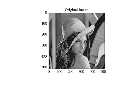
When  correlate and/or convolve can be used
to construct arbitrary image filters to perform actions such as blurring,
enhancing, and edge-detection for an image.
correlate and/or convolve can be used
to construct arbitrary image filters to perform actions such as blurring,
enhancing, and edge-detection for an image.
>>> import numpy as np
>>> from scipy import signal, misc
>>> import matplotlib.pyplot as plt
>>> image = misc.lena()
>>> w = np.zeros((50, 50))
>>> w[0][0] = 1.0
>>> w[49][25] = 1.0
>>> image_new = signal.fftconvolve(image, w)
>>> plt.figure()
>>> plt.imshow(image)
>>> plt.gray()
>>> plt.title('Original image')
>>> plt.show()
>>> plt.figure()
>>> plt.imshow(image_new)
>>> plt.gray()
>>> plt.title('Filtered image')
>>> plt.show()
Using convolve in the above example would take quite long to run.
Calculating the convolution in the time domain as above is mainly used for
filtering when one of the signals is much smaller than the other (  ), otherwise linear filtering is more efficiently calculated in the
frequency domain provided by the function fftconvolve.
), otherwise linear filtering is more efficiently calculated in the
frequency domain provided by the function fftconvolve.
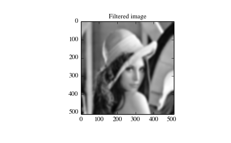
If the filter function ![w[n,m]](../_images/math/c78dbc10d70a889d9fefc9dc12f36e56b118b7a5.png) can be factored according to
can be factored according to
![h[n, m] = h_1[n] h_2[m],](../_images/math/4f18fc3b9ac6ff2b93353e74554bc3c62c323efb.png)
convolution can be calculated by means of the function sepfir2d. As an example we consider a Gaussian filter gaussian
![h[n, m] \propto e^{-x^2-y^2} = e^{-x^2} e^{-y^2}](../_images/math/e1bfc06e59a492a0b5e3ffac5dee2b60a950aa51.png)
which is often used for blurring.
>>> import numpy as np
>>> from scipy import signal, misc
>>> import matplotlib.pyplot as plt
>>> image = misc.lena()
>>> w = signal.gaussian(50, 5.0)
>>> image_new = signal.sepfir2d(image, w, w)
>>> plt.figure()
>>> plt.imshow(image)
>>> plt.gray()
>>> plt.title('Original image')
>>> plt.show()

>>> plt.figure()
>>> plt.imshow(image_new)
>>> plt.gray()
>>> plt.title('Filtered image')
>>> plt.show()
Difference-equation filtering
A general class of linear one-dimensional filters (that includes convolution filters) are filters described by the difference equation
![\sum_{k=0}^{N}a_{k}y\left[n-k\right]=\sum_{k=0}^{M}b_{k}x\left[n-k\right]](../_images/math/cdf9add6a4c5e0f80116123ac0f49b5df2c0bfd7.png)
where is the input sequence and
![y\left[n\right]](../_images/math/ac05524a8e63d5ccd924e7f512fd160cda158742.png) is the output sequence. If we assume initial rest so
that for
is the output sequence. If we assume initial rest so
that for  , then this kind of filter can
be implemented using convolution. However, the convolution filter sequence
, then this kind of filter can
be implemented using convolution. However, the convolution filter sequence
![h\left[n\right]](../_images/math/d84e7ee45c89f90b2a18a15a666a549a73989ed0.png) could be infinite if
could be infinite if  for
for
 In addition, this general class of linear filter allows
initial conditions to be placed on for
resulting in a filter that cannot be expressed using convolution.
In addition, this general class of linear filter allows
initial conditions to be placed on for
resulting in a filter that cannot be expressed using convolution.
The difference equation filter can be thought of as finding
recursively in terms of it’s previous values
![a_{0}y\left[n\right]=-a_{1}y\left[n-1\right]-\cdots-a_{N}y\left[n-N\right]+\cdots+b_{0}x\left[n\right]+\cdots+b_{M}x\left[n-M\right].](../_images/math/4fede67438d84061feb4be59d6edffc172f859da.png)
Often  is chosen for normalization. The implementation in SciPy
of this general difference equation filter is a little more complicated then
would be implied by the previous equation. It is implemented so that only one
signal needs to be delayed. The actual implementation equations are (assuming
).
is chosen for normalization. The implementation in SciPy
of this general difference equation filter is a little more complicated then
would be implied by the previous equation. It is implemented so that only one
signal needs to be delayed. The actual implementation equations are (assuming
).
![\begin{eqnarray*} y\left[n\right] & = & b_{0}x\left[n\right]+z_{0}\left[n-1\right]\\ z_{0}\left[n\right] & = & b_{1}x\left[n\right]+z_{1}\left[n-1\right]-a_{1}y\left[n\right]\\ z_{1}\left[n\right] & = & b_{2}x\left[n\right]+z_{2}\left[n-1\right]-a_{2}y\left[n\right]\\ \vdots & \vdots & \vdots\\ z_{K-2}\left[n\right] & = & b_{K-1}x\left[n\right]+z_{K-1}\left[n-1\right]-a_{K-1}y\left[n\right]\\ z_{K-1}\left[n\right] & = & b_{K}x\left[n\right]-a_{K}y\left[n\right],\end{eqnarray*}](../_images/math/6099144fb3e1c3bf28f34400275f1e93188edc18.png)
where  Note that
  if
if  and
and  if
if  In this way, the output at time
  depends only on the input at time and the value of
  at
the previous time. This can always be calculated as long as the
values
at
the previous time. This can always be calculated as long as the
values ![z_{0}\left[n-1\right]\ldots z_{K-1}\left[n-1\right]](../_images/math/42f1f614b9334d3b742116f2e7ee66fb4abac310.png) are
computed and stored at each time step.
are
computed and stored at each time step.
The difference-equation filter is called using the command lfilter in
SciPy. This command takes as inputs the vector  the vector,
 a signal and returns the vector (the same
length as ) computed using the equation given above. If is
-dimensional, then the filter is computed along the axis provided.
If, desired, initial conditions providing the values of
a signal and returns the vector (the same
length as ) computed using the equation given above. If is
-dimensional, then the filter is computed along the axis provided.
If, desired, initial conditions providing the values of
![z_{0}\left[-1\right]](../_images/math/43ab2eed734f96551ceb27ef0fcbd4199738fe93.png) to
to ![z_{K-1}\left[-1\right]](../_images/math/b7a60fd83d0a87028ce08ab9ffa630f620e88765.png) can be provided
or else it will be assumed that they are all zero. If initial conditions are
provided, then the final conditions on the intermediate variables are also
returned. These could be used, for example, to restart the calculation in the
same state.
can be provided
or else it will be assumed that they are all zero. If initial conditions are
provided, then the final conditions on the intermediate variables are also
returned. These could be used, for example, to restart the calculation in the
same state.
Sometimes it is more convenient to express the initial conditions in terms of
the signals and ![y\left[n\right].](../_images/math/a2046cdd0206b97fb1a930ee4ceb7fb698d11c0b.png) In other
words, perhaps you have the values of
In other
words, perhaps you have the values of ![x\left[-M\right]](../_images/math/37e5088386bdaf6061ee2e211dab9e6022ed48e5.png) to
to
![x\left[-1\right]](../_images/math/5d44f008323427729b43050707ae9aac27ef0501.png) and the values of
and the values of ![y\left[-N\right]](../_images/math/65d990cf6d6c8c546d85620b4450ac076b7d0aca.png) to
to
![y\left[-1\right]](../_images/math/e5a86a26e33ab28a922d81e17456ade6799d83f8.png) and would like to determine what values of
and would like to determine what values of
![z_{m}\left[-1\right]](../_images/math/60cf99b53ac74d8571129966cb3693355609614e.png) should be delivered as initial conditions to the
difference-equation filter. It is not difficult to show that for
should be delivered as initial conditions to the
difference-equation filter. It is not difficult to show that for 
![z_{m}\left[n\right]=\sum_{p=0}^{K-m-1}\left(b_{m+p+1}x\left[n-p\right]-a_{m+p+1}y\left[n-p\right]\right).](../_images/math/10c2b866ee8c90ee0b3cabdb9645b0a9eca4194d.png)
Using this formula we can find the initial condition vector
to given initial
conditions on (and ). The command lfiltic performs
this function.
As an example consider the following system:
![y[n] = \frac{1}{2} x[n] + \frac{1}{4} x[n-1] + \frac{1}{3} y[n-1]](../_images/math/67092b9b7c642f34cbb47f3f05088ea3cc91e810.png)
The code calculates the signal ![y[n]](../_images/math/b0305c23171428d437153e26d595c82ef3df240a.png) for a given signal
for a given signal ![x[n]](../_images/math/1c7654440717b398fc6aa2479be47978c0cae90b.png) ;
first for initial condiditions
;
first for initial condiditions ![y[-1] = 0](../_images/math/58efefd959e61db0a6a207e6bb03c800e181852d.png) (default case), then for
(default case), then for
![y[-1] = 2](../_images/math/813a2b40fe24a08eeff9810261ee8e385cd2eaa5.png) by means of :fun:`lfiltic`.
by means of :fun:`lfiltic`.
>>> import numpy as np
>>> from scipy import signal
>>> x = np.array([1., 0., 0., 0.])
>>> b = np.array([1.0/2, 1.0/4])
>>> a = np.array([1.0, -1.0/3])
>>> signal.lfilter(b, a, x)
[ 0.5         0.41666667  0.13888889  0.0462963 ]
>>> zi = signal.lfiltic(b, a, y=[2.])
>>> signal.lfilter(b, a, x, zi=zi)
[ 1.16666667,  0.63888889,  0.21296296,  0.07098765]
Note that the output signal has the same length as the length as
the input signal .
Analysis of Linear Systems
Linear system described a linear difference equation can be fully described by
the coefficient vectors a and b as was done above; an alternative
representation is to provide a factor  ,
,  zeros
zeros  and
and  poles
poles  , respectively, to describe the system by
means of its transfer function
, respectively, to describe the system by
means of its transfer function  according to
This alternative representation can be obtain wit hthe scipy function tf2zpk; the inverse is provided by zpk2tf.
For the example from above we have
>>> b = np.array([1.0/2, 1.0/4])
>>> a = np.array([1.0, -1.0/3])
>>> signal.tf2zpk(b, a)
[-0.5] [ 0.33333333] 0.5
i.e. the system has a zero at  and a pole at
  .
.
The scipy function freqz allows calculation of the frequency response
of a system described by the coeffcients  and
and  . See the
help of the freqz function of a comprehensive example.
. See the
help of the freqz function of a comprehensive example.
Filter Design
Time-discrete filters can be classified into finite response (FIR) filters and infinite response (IIR) filters. FIR filters provide a linear phase response, whereas IIR filters do not exhibit this behaviour. Scipy provides functions for designing both types of filters.
FIR Filter
The function firwin designs filters according to the window method. Depending on the provided arguments, the function returns different filter types (e.g. low-pass, band-pass...).
The example below designs a low-pass and a band-stop filter, respectively.
>>> import numpy as np
>>> import scipy.signal as signal
>>> import matplotlib.pyplot as plt
>>> b1 = signal.firwin(40, 0.5)
>>> b2 = signal.firwin(41, [0.3, 0.8])
>>> w1, h1 = signal.freqz(b1)
>>> w2, h2 = signal.freqz(b2)
>>> plt.title('Digital filter frequency response')
>>> plt.plot(w1, 20*np.log10(np.abs(h1)), 'b')
>>> plt.plot(w2, 20*np.log10(np.abs(h2)), 'r')
>>> plt.ylabel('Amplitude Response (dB)')
>>> plt.xlabel('Frequency (rad/sample)')
>>> plt.grid()
>>> plt.show()
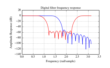
Note that firwin uses per default a normalized frequency defined such
that the value  corresponds to the Nyquist frequency, whereas the
function freqz is defined such that the value
corresponds to the Nyquist frequency, whereas the
function freqz is defined such that the value  corresponds
to the Nyquist frequency.
corresponds
to the Nyquist frequency.
The function firwin2 allows design of almost arbitrary frequency responses by specifying an array of corner frequencies and corresponding gains, respectively.
The example below designs a filter with such an arbitrary amplitude response.
>>> import numpy as np
>>> import scipy.signal as signal
>>> import matplotlib.pyplot as plt
>>> b = signal.firwin2(150, [0.0, 0.3, 0.6, 1.0], [1.0, 2.0, 0.5, 0.0])
>>> w, h = signal.freqz(b)
>>> plt.title('Digital filter frequency response')
>>> plt.plot(w, np.abs(h))
>>> plt.title('Digital filter frequency response')
>>> plt.ylabel('Amplitude Response')
>>> plt.xlabel('Frequency (rad/sample)')
>>> plt.grid()
>>> plt.show()
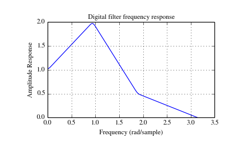
Note the linear scaling of the y-axis and the different definition of the Nyquist frequency in firwin2 and freqz (as explained above).
IIR Filter
Scipy provides two functions to directly design IIR iirdesign and iirfilter where the filter type (e.g. elliptic) is passed as an argument and several more filter design functions for specific filter types; e.g. ellip.
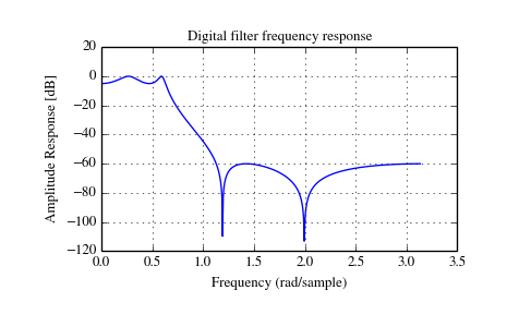
The example below designs an elliptic low-pass filter with defined passband
and stopband ripple, respectively. Note the much lower filter order (order 4)
compared with the FIR filters from the examples above in order to reach the same
stop-band attenuation of  dB.
dB.
>>> import numpy as np
>>> import scipy.signal as signal
>>> import matplotlib.pyplot as plt
>>> b, a = signal.iirfilter(4, Wn=0.2, rp=5, rs=60, btype='lowpass', ftype='ellip')
>>> w, h = signal.freqz(b, a)
>>> plt.title('Digital filter frequency response')
>>> plt.plot(w, 20*np.log10(np.abs(h)))
>>> plt.title('Digital filter frequency response')
>>> plt.ylabel('Amplitude Response [dB]')
>>> plt.xlabel('Frequency (rad/sample)')
>>> plt.grid()
>>> plt.show()
Other filters
The signal processing package provides many more filters as well.
Median Filter
A median filter is commonly applied when noise is markedly non-Gaussian or when it is desired to preserve edges. The median filter works by sorting all of the array pixel values in a rectangular region surrounding the point of interest. The sample median of this list of neighborhood pixel values is used as the value for the output array. The sample median is the middle array value in a sorted list of neighborhood values. If there are an even number of elements in the neighborhood, then the average of the middle two values is used as the median. A general purpose median filter that works on N-dimensional arrays is medfilt . A specialized version that works only for two-dimensional arrays is available as medfilt2d .
Order Filter
A median filter is a specific example of a more general class of filters called order filters. To compute the output at a particular pixel, all order filters use the array values in a region surrounding that pixel. These array values are sorted and then one of them is selected as the output value. For the median filter, the sample median of the list of array values is used as the output. A general order filter allows the user to select which of the sorted values will be used as the output. So, for example one could choose to pick the maximum in the list or the minimum. The order filter takes an additional argument besides the input array and the region mask that specifies which of the elements in the sorted list of neighbor array values should be used as the output. The command to perform an order filter is order_filter.
Wiener filter
The Wiener filter is a simple deblurring filter for denoising images. This is
not the Wiener filter commonly described in image reconstruction problems but
instead it is a simple, local-mean filter. Let be the input signal,
then the output is
where  is the local estimate of the mean and
 is the local estimate of the variance. The window for
these estimates is an optional input parameter (default is
is the local estimate of the variance. The window for
these estimates is an optional input parameter (default is  ).
The parameter
).
The parameter  is a threshold noise parameter. If
 is not given then it is estimated as the average of the local
variances.
is not given then it is estimated as the average of the local
variances.
Hilbert filter
The Hilbert transform constructs the complex-valued analytic signal
from a real signal. For example if  then
then
 would return (except near the
edges)
would return (except near the
edges)  In the frequency domain,
the hilbert transform performs
In the frequency domain,
the hilbert transform performs

where  is 2 for positive frequencies,
  for negative
frequencies and for zero-frequencies.
for negative
frequencies and for zero-frequencies.
Analog Filter Design
The functions iirdesign, iirfilter, and the filter design functions for specific filter types (e.g. ellip) all have a flag analog which allows design of analog filters as well.
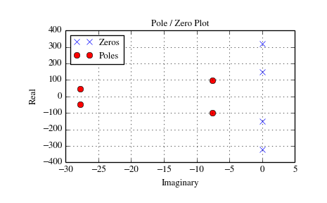
The example below designs an analog (IIR) filter, obtains via tf2zpk
the poles and zeros and plots them in the complex s-plane. The zeros at
 and
and  can be clearly seen
in the amplitude response.
can be clearly seen
in the amplitude response.
>>> import numpy as np
>>> import scipy.signal as signal
>>> import matplotlib.pyplot as plt
>>> b, a = signal.iirdesign(wp=100, ws=200, gpass=2.0, gstop=40., analog=True)
>>> w, h = signal.freqs(b, a)
>>> plt.title('Analog filter frequency response')
>>> plt.plot(w, 20*np.log10(np.abs(h)))
>>> plt.ylabel('Amplitude Response [dB]')
>>> plt.xlabel('Frequency')
>>> plt.grid()
>>> plt.show()

>>> z, p, k = signal.tf2zpk(b, a)
>>> plt.plot(np.real(z), np.imag(z), 'xb')
>>> plt.plot(np.real(p), np.imag(p), 'or')
>>> plt.legend(['Zeros', 'Poles'], loc=2)
>>> plt.title('Pole / Zero Plot')
>>> plt.ylabel('Real')
>>> plt.xlabel('Imaginary')
>>> plt.grid()
>>> plt.show()
Spectral Analysis
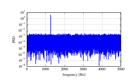
Periodogram Measurements
The scipy function periodogram provides a method to estimate the spectral density using the periodogram method.
The example below calculates the periodogram of a sine signal in white Gaussian noise.
>>> import numpy as np
>>> import scipy.signal as signal
>>> import matplotlib.pyplot as plt
>>> fs = 10e3
>>> N = 1e5
>>> amp = 2*np.sqrt(2)
>>> freq = 1270.0
>>> noise_power = 0.001 * fs / 2
>>> time = np.arange(N) / fs
>>> x = amp*np.sin(2*np.pi*freq*time)
>>> x += np.random.normal(scale=np.sqrt(noise_power), size=time.shape)
>>> f, Pper_spec = signal.periodogram(x, fs, 'flattop', scaling='spectrum')
>>> plt.semilogy(f, Pper_spec)
>>> plt.xlabel('frequency [Hz]')
>>> plt.ylabel('PSD')
>>> plt.grid()
>>> plt.show()
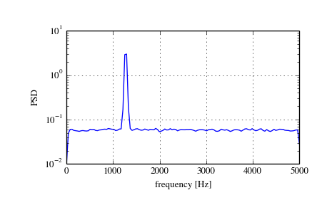
Spectral Analysis using Welch’s Method
An improved method, especially with respect to noise immunity, is Welch’s method which is implemented by the scipy function welch.
The example below estimates the spectrum using Welch’s method and uses the same parameters as the example above. Note the much smoother noise floor of the spectogram.
>>> import numpy as np
>>> import scipy.signal as signal
>>> import matplotlib.pyplot as plt
>>> fs = 10e3
>>> N = 1e5
>>> amp = 2*np.sqrt(2)
>>> freq = 1270.0
>>> noise_power = 0.001 * fs / 2
>>> time = np.arange(N) / fs
>>> x = amp*np.sin(2*np.pi*freq*time)
>>> x += np.random.normal(scale=np.sqrt(noise_power), size=time.shape)
>>> f, Pwelch_spec = signal.welch(x, fs, scaling='spectrum')
>>> plt.semilogy(f, Pwelch_spec)
>>> plt.xlabel('frequency [Hz]')
>>> plt.ylabel('PSD')
>>> plt.grid()
>>> plt.show()
Lomb-Scargle Periodograms (lombscargle)
Least-squares spectral analysis (LSSA) is a method of estimating a frequency spectrum, based on a least squares fit of sinusoids to data samples, similar to Fourier analysis. Fourier analysis, the most used spectral method in science, generally boosts long-periodic noise in long gapped records; LSSA mitigates such problems.
The Lomb-Scargle method performs spectral analysis on unevenly sampled data and is known to be a powerful way to find, and test the significance of, weak periodic signals.
For a time series comprising  measurements
  sampled at times
  where
where  ,
assumed to have been scaled and shifted such that its mean is zero and its
variance is unity, the normalized Lomb-Scargle periodogram at frequency
,
assumed to have been scaled and shifted such that its mean is zero and its
variance is unity, the normalized Lomb-Scargle periodogram at frequency
 is
is
![P_{n}(f) \frac{1}{2}\left\{\frac{\left[\sum_{j}^{N_{t}}X_{j}\cos\omega(t_{j}-\tau)\right]^{2}}{\sum_{j}^{N_{t}}\cos^{2}\omega(t_{j}-\tau)}+\frac{\left[\sum_{j}^{N_{t}}X_{j}\sin\omega(t_{j}-\tau)\right]^{2}}{\sum_{j}^{N_{t}}\sin^{2}\omega(t_{j}-\tau)}\right\}.](../_images/math/fe38fc8e276e35c41ed994b484ad41eedb8c5888.png)
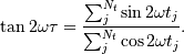
Here,  is the angular frequency. The frequency
dependent time offset
is the angular frequency. The frequency
dependent time offset  is given by
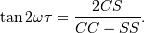
The lombscargle function calculates the periodogram using a slightly modified algorithm due to Townsend [3] which allows the periodogram to be calculated using only a single pass through the input arrays for each frequency.
The equation is refactored as:
![P_{n}(f) = \frac{1}{2}\left[\frac{(c_{\tau}XC + s_{\tau}XS)^{2}}{c_{\tau}^{2}CC + 2c_{\tau}s_{\tau}CS + s_{\tau}^{2}SS} + \frac{(c_{\tau}XS - s_{\tau}XC)^{2}}{c_{\tau}^{2}SS - 2c_{\tau}s_{\tau}CS + s_{\tau}^{2}CC}\right]](../_images/math/ce30ef4da64785a03fa7c931a9bed4e1ee47af4a.png)
and
Here,

while the sums are
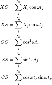
This requires  trigonometric function evaluations
giving a factor of
trigonometric function evaluations
giving a factor of  speed increase over the straightforward
implementation.
speed increase over the straightforward
implementation.
Detrend
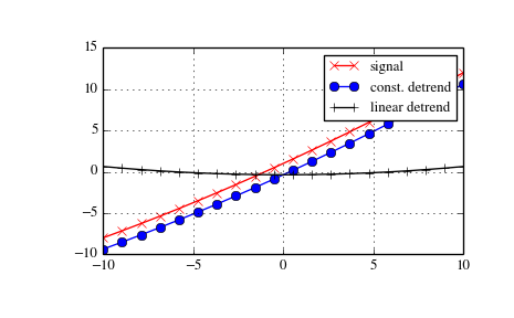
Scipy provides the function detrend to remove a constant or linear trend in a data series in order to see effect of higher order.
The example below removes the constant and linear trend of a 2-nd order polynomial time series and plots the remaining signal components.
>>> import numpy as np
>>> import scipy.signal as signal
>>> import matplotlib.pyplot as plt
>>> t = np.linspace(-10, 10, 20)
>>> y = 1 + t + 0.01*t**2
>>> yconst = signal.detrend(y, type='constant')
>>> ylin = signal.detrend(y, type='linear')
>>> plt.plot(t, y, '-rx')
>>> plt.plot(t, yconst, '-bo')
>>> plt.plot(t, ylin, '-k+')
>>> plt.grid()
>>> plt.legend(['signal', 'const. detrend', 'linear detrend'])
>>> plt.show()
References
Some further reading and related software:
| [1] | N.R. Lomb “Least-squares frequency analysis of unequally spaced data”, Astrophysics and Space Science, vol 39, pp. 447-462, 1976 |
| [2] | J.D. Scargle “Studies in astronomical time series analysis. II - Statistical aspects of spectral analysis of unevenly spaced data”, The Astrophysical Journal, vol 263, pp. 835-853, 1982 |
| [3] | R.H.D. Townsend, “Fast calculation of the Lomb-Scargle periodogram using graphics processing units.”, The Astrophysical Journal Supplement Series, vol 191, pp. 247-253, 2010 |