scipy.signal.cwt#

scipy.signal.cwt(data, wavelet, widths, dtype=None, **kwargs)[source]#

Continuous wavelet transform.

Performs a continuous wavelet transform on data, using the wavelet function. A CWT performs a convolution with data using the wavelet function, which is characterized by a width parameter and length parameter. The wavelet function is allowed to be complex.

Parameters

data(N,) ndarray: data on which to perform the transform.
waveletfunction: Wavelet function, which should take 2 arguments. The first argument is the number of points that the returned vector will have (len(wavelet(length,width)) == length). The second is a width parameter, defining the size of the wavelet (e.g. standard deviation of a gaussian). See ricker, which satisfies these requirements.
widths(M,) sequence: Widths to use for transform.
dtypedata-type, optional: The desired data type of output. Defaults to float64 if the output of wavelet is real and complex128 if it is complex.

New in version 1.4.0.
kwargs: Keyword arguments passed to wavelet function.

New in version 1.4.0.

Returns

cwt: (M, N) ndarray: Will have shape of (len(widths), len(data)).

Notes

New in version 1.4.0.

For non-symmetric, complex-valued wavelets, the input signal is convolved with the time-reversed complex-conjugate of the wavelet data [1].

length = min(10 * width[ii], len(data))
cwt[ii,:] = signal.convolve(data, np.conj(wavelet(length, width[ii],
                                **kwargs))[::-1], mode='same')

References

1: S. Mallat, “A Wavelet Tour of Signal Processing (3rd Edition)”, Academic Press, 2009.

Examples

>>> from scipy import signal
>>> import matplotlib.pyplot as plt
>>> t = np.linspace(-1, 1, 200, endpoint=False)
>>> sig  = np.cos(2 * np.pi * 7 * t) + signal.gausspulse(t - 0.4, fc=2)
>>> widths = np.arange(1, 31)
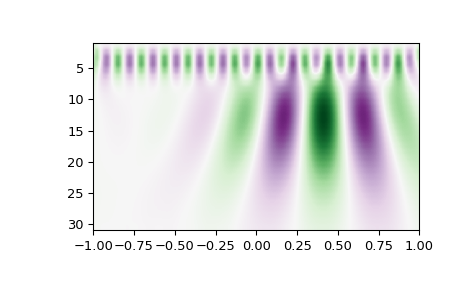
>>> cwtmatr = signal.cwt(sig, signal.ricker, widths)
>>> plt.imshow(cwtmatr, extent=[-1, 1, 31, 1], cmap='PRGn', aspect='auto',
...            vmax=abs(cwtmatr).max(), vmin=-abs(cwtmatr).max())
>>> plt.show()