scipy.optimize.rosen#
- scipy.optimize.rosen(x)[source]#
The Rosenbrock function.
The function computed is:
sum(100.0*(x[1:] - x[:-1]**2.0)**2.0 + (1 - x[:-1])**2.0)
- Parameters
- xarray_like
1-D array of points at which the Rosenbrock function is to be computed.
- Returns
- ffloat
The value of the Rosenbrock function.
See also
Examples
>>> from scipy.optimize import rosen
>>> X = 0.1 * np.arange(10)
>>> rosen(X)
76.56
For higher-dimensional input
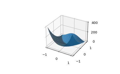
rosenbroadcasts. In the following example, we use this to plot a 2D landscape. Note thatrosen_hessdoes not broadcast in this manner.>>> import matplotlib.pyplot as plt >>> from mpl_toolkits.mplot3d import Axes3D >>> x = np.linspace(-1, 1, 50) >>> X, Y = np.meshgrid(x, x) >>> ax = plt.subplot(111, projection='3d') >>> ax.plot_surface(X, Y, rosen([X, Y])) >>> plt.show()
