scipy.integrate.solve_bvp

scipy.integrate.solve_bvp(fun, bc, x, y, p=None, S=None, fun_jac=None, bc_jac=None, tol=0.001, max_nodes=1000, verbose=0, bc_tol=None)

Solve a boundary value problem for a system of ODEs.

This function numerically solves a first order system of ODEs subject to two-point boundary conditions:

dy / dx = f(x, y, p) + S * y / (x - a), a <= x <= b
bc(y(a), y(b), p) = 0

Here x is a 1-D independent variable, y(x) is an N-D vector-valued function and p is a k-D vector of unknown parameters which is to be found along with y(x). For the problem to be determined, there must be n + k boundary conditions, i.e., bc must be an (n + k)-D function.

The last singular term on the right-hand side of the system is optional. It is defined by an n-by-n matrix S, such that the solution must satisfy S y(a) = 0. This condition will be forced during iterations, so it must not contradict boundary conditions. See [2] for the explanation how this term is handled when solving BVPs numerically.

Problems in a complex domain can be solved as well. In this case, y and p are considered to be complex, and f and bc are assumed to be complex-valued functions, but x stays real. Note that f and bc must be complex differentiable (satisfy Cauchy-Riemann equations [4]), otherwise you should rewrite your problem for real and imaginary parts separately. To solve a problem in a complex domain, pass an initial guess for y with a complex data type (see below).

Parameters

funcallable

Right-hand side of the system. The calling signature is fun(x, y), or fun(x, y, p) if parameters are present. All arguments are ndarray: x with shape (m,), y with shape (n, m), meaning that y[:, i] corresponds to x[i], and p with shape (k,). The return value must be an array with shape (n, m) and with the same layout as y.

bccallable

Function evaluating residuals of the boundary conditions. The calling signature is bc(ya, yb), or bc(ya, yb, p) if parameters are present. All arguments are ndarray: ya and yb with shape (n,), and p with shape (k,). The return value must be an array with shape (n + k,).

xarray_like, shape (m,)

Initial mesh. Must be a strictly increasing sequence of real numbers with x[0]=a and x[-1]=b.

yarray_like, shape (n, m)

Initial guess for the function values at the mesh nodes, ith column corresponds to x[i]. For problems in a complex domain pass y with a complex data type (even if the initial guess is purely real).

parray_like with shape (k,) or None, optional

Initial guess for the unknown parameters. If None (default), it is assumed that the problem doesn’t depend on any parameters.

Sarray_like with shape (n, n) or None

Matrix defining the singular term. If None (default), the problem is solved without the singular term.

fun_jaccallable or None, optional

Function computing derivatives of f with respect to y and p. The calling signature is fun_jac(x, y), or fun_jac(x, y, p) if parameters are present. The return must contain 1 or 2 elements in the following order:

• df_dy : array_like with shape (n, n, m), where an element (i, j, q) equals to d f_i(x_q, y_q, p) / d (y_q)_j.

• df_dp : array_like with shape (n, k, m), where an element (i, j, q) equals to d f_i(x_q, y_q, p) / d p_j.

Here q numbers nodes at which x and y are defined, whereas i and j number vector components. If the problem is solved without unknown parameters, df_dp should not be returned.

If fun_jac is None (default), the derivatives will be estimated by the forward finite differences.

bc_jaccallable or None, optional

Function computing derivatives of bc with respect to ya, yb, and p. The calling signature is bc_jac(ya, yb), or bc_jac(ya, yb, p) if parameters are present. The return must contain 2 or 3 elements in the following order:

• dbc_dya : array_like with shape (n, n), where an element (i, j) equals to d bc_i(ya, yb, p) / d ya_j.

• dbc_dyb : array_like with shape (n, n), where an element (i, j) equals to d bc_i(ya, yb, p) / d yb_j.

• dbc_dp : array_like with shape (n, k), where an element (i, j) equals to d bc_i(ya, yb, p) / d p_j.

If the problem is solved without unknown parameters, dbc_dp should not be returned.

If bc_jac is None (default), the derivatives will be estimated by the forward finite differences.

tolfloat, optional

Desired tolerance of the solution. If we define r = y' - f(x, y), where y is the found solution, then the solver tries to achieve on each mesh interval norm(r / (1 + abs(f)) < tol, where norm is estimated in a root mean squared sense (using a numerical quadrature formula). Default is 1e-3.

max_nodesint, optional

Maximum allowed number of the mesh nodes. If exceeded, the algorithm terminates. Default is 1000.

verbose{0, 1, 2}, optional

Level of algorithm’s verbosity:

• 0 (default) : work silently.

• 1 : display a termination report.

• 2 : display progress during iterations.

bc_tolfloat, optional

Desired absolute tolerance for the boundary condition residuals: bc value should satisfy abs(bc) < bc_tol component-wise. Equals to tol by default. Up to 10 iterations are allowed to achieve this tolerance.

Returns

Bunch object with the following fields defined:

solPPoly

Found solution for y as scipy.interpolate.PPoly instance, a C1 continuous cubic spline.

pndarray or None, shape (k,)

Found parameters. None, if the parameters were not present in the problem.

xndarray, shape (m,)

Nodes of the final mesh.

yndarray, shape (n, m)

Solution values at the mesh nodes.

ypndarray, shape (n, m)

Solution derivatives at the mesh nodes.

rms_residualsndarray, shape (m - 1,)

RMS values of the relative residuals over each mesh interval (see the description of tol parameter).

niterint

Number of completed iterations.

statusint

Reason for algorithm termination:

• 0: The algorithm converged to the desired accuracy.

• 1: The maximum number of mesh nodes is exceeded.

• 2: A singular Jacobian encountered when solving the collocation system.

messagestring

Verbal description of the termination reason.

successbool

True if the algorithm converged to the desired accuracy (status=0).

Notes

This function implements a 4th order collocation algorithm with the control of residuals similar to [1]. A collocation system is solved by a damped Newton method with an affine-invariant criterion function as described in [3].

Note that in [1] integral residuals are defined without normalization by interval lengths. So, their definition is different by a multiplier of h**0.5 (h is an interval length) from the definition used here.

New in version 0.18.0.

References

1(1,2)

J. Kierzenka, L. F. Shampine, “A BVP Solver Based on Residual Control and the Maltab PSE”, ACM Trans. Math. Softw., Vol. 27, Number 3, pp. 299-316, 2001.

2

L.F. Shampine, P. H. Muir and H. Xu, “A User-Friendly Fortran BVP Solver”.

3

U. Ascher, R. Mattheij and R. Russell “Numerical Solution of Boundary Value Problems for Ordinary Differential Equations”.

4

Cauchy-Riemann equations on Wikipedia.

Examples

In the first example, we solve Bratu’s problem:

y'' + k * exp(y) = 0
y(0) = y(1) = 0

for k = 1.

We rewrite the equation as a first-order system and implement its right-hand side evaluation:

y1' = y2
y2' = -exp(y1)

>>> def fun(x, y):
...     return np.vstack((y[1], -np.exp(y[0])))

Implement evaluation of the boundary condition residuals:

>>> def bc(ya, yb):
...     return np.array([ya[0], yb[0]])

Define the initial mesh with 5 nodes:

>>> x = np.linspace(0, 1, 5)

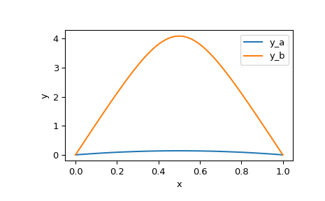
This problem is known to have two solutions. To obtain both of them, we use two different initial guesses for y. We denote them by subscripts a and b.

>>> y_a = np.zeros((2, x.size))
>>> y_b = np.zeros((2, x.size))
>>> y_b[0] = 3

Now we are ready to run the solver.

>>> from scipy.integrate import solve_bvp
>>> res_a = solve_bvp(fun, bc, x, y_a)
>>> res_b = solve_bvp(fun, bc, x, y_b)

Let’s plot the two found solutions. We take an advantage of having the solution in a spline form to produce a smooth plot.

>>> x_plot = np.linspace(0, 1, 100)
>>> y_plot_a = res_a.sol(x_plot)[0]
>>> y_plot_b = res_b.sol(x_plot)[0]
>>> import matplotlib.pyplot as plt
>>> plt.plot(x_plot, y_plot_a, label='y_a')
>>> plt.plot(x_plot, y_plot_b, label='y_b')
>>> plt.legend()
>>> plt.xlabel("x")
>>> plt.ylabel("y")
>>> plt.show()

We see that the two solutions have similar shape, but differ in scale significantly.

In the second example, we solve a simple Sturm-Liouville problem:

y'' + k**2 * y = 0
y(0) = y(1) = 0

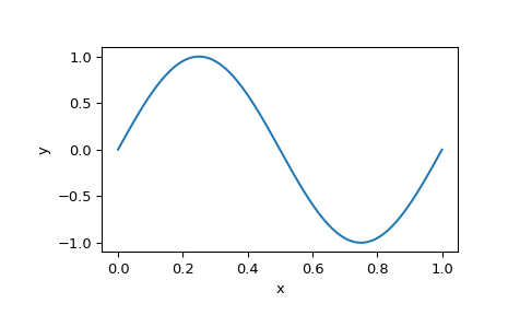
It is known that a non-trivial solution y = A * sin(k * x) is possible for k = pi * n, where n is an integer. To establish the normalization constant A = 1 we add a boundary condition:

y'(0) = k

Again, we rewrite our equation as a first-order system and implement its right-hand side evaluation:

y1' = y2
y2' = -k**2 * y1

>>> def fun(x, y, p):
...     k = p[0]
...     return np.vstack((y[1], -k**2 * y[0]))

Note that parameters p are passed as a vector (with one element in our case).

Implement the boundary conditions:

>>> def bc(ya, yb, p):
...     k = p[0]
...     return np.array([ya[0], yb[0], ya[1] - k])

Set up the initial mesh and guess for y. We aim to find the solution for k = 2 * pi, to achieve that we set values of y to approximately follow sin(2 * pi * x):

>>> x = np.linspace(0, 1, 5)
>>> y = np.zeros((2, x.size))
>>> y[0, 1] = 1
>>> y[0, 3] = -1

Run the solver with 6 as an initial guess for k.

>>> sol = solve_bvp(fun, bc, x, y, p=[6])

We see that the found k is approximately correct:

>>> sol.p[0]
6.28329460046

And, finally, plot the solution to see the anticipated sinusoid:

>>> x_plot = np.linspace(0, 1, 100)
>>> y_plot = sol.sol(x_plot)[0]
>>> plt.plot(x_plot, y_plot)
>>> plt.xlabel("x")
>>> plt.ylabel("y")
>>> plt.show()