scipy.stats.linregress
-
scipy.stats.linregress(x, y=None)[source]¶ Calculate a linear least-squares regression for two sets of measurements.
- Parameters
- x, yarray_like
Two sets of measurements. Both arrays should have the same length. If only x is given (and
y=None), then it must be a two-dimensional array where one dimension has length 2. The two sets of measurements are then found by splitting the array along the length-2 dimension. In the case wherey=Noneand x is a 2x2 array,linregress(x)is equivalent tolinregress(x[0], x[1]).
- Returns
- result
LinregressResultinstance The return value is an object with the following attributes:
- slopefloat
Slope of the regression line.
- interceptfloat
Intercept of the regression line.
- rvaluefloat
Correlation coefficient.
- pvaluefloat
Two-sided p-value for a hypothesis test whose null hypothesis is that the slope is zero, using Wald Test with t-distribution of the test statistic.
- stderrfloat
Standard error of the estimated slope (gradient), under the assumption of residual normality.
- intercept_stderrfloat
Standard error of the estimated intercept, under the assumption of residual normality.
- result
See also
scipy.optimize.curve_fitUse non-linear least squares to fit a function to data.
scipy.optimize.leastsqMinimize the sum of squares of a set of equations.
Notes
Missing values are considered pair-wise: if a value is missing in x, the corresponding value in y is masked.
For compatibility with older versions of SciPy, the return value acts like a
namedtupleof length 5, with fieldsslope,intercept,rvalue,pvalueandstderr, so one can continue to write:slope, intercept, r, p, se = linregress(x, y)
With that style, however, the standard error of the intercept is not available. To have access to all the computed values, including the standard error of the intercept, use the return value as an object with attributes, e.g.:
result = linregress(x, y)
print(result.intercept, result.intercept_stderr)
Examples
>>> import matplotlib.pyplot as plt
>>> from scipy import stats
Generate some data:
>>> np.random.seed(12345678)
>>> x = np.random.random(10)
>>> y = 1.6*x + np.random.random(10)
Perform the linear regression:
>>> res = stats.linregress(x, y)
Coefficient of determination (R-squared):
>>> print(f"R-squared: {res.rvalue**2:.6f}")
R-squared: 0.735498
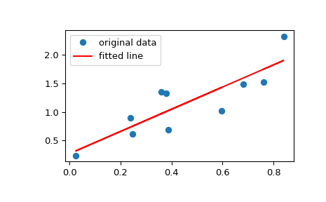
Plot the data along with the fitted line:
>>> plt.plot(x, y, 'o', label='original data')
>>> plt.plot(x, res.intercept + res.slope*x, 'r', label='fitted line')
>>> plt.legend()
>>> plt.show()
Calculate 95% confidence interval on slope and intercept:
>>> # Two-sided inverse Students t-distribution
>>> # p - probability, df - degrees of freedom
>>> from scipy.stats import t
>>> tinv = lambda p, df: abs(t.ppf(p/2, df))
>>> ts = tinv(0.05, len(x)-2)
>>> print(f"slope (95%): {res.slope:.6f} +/- {ts*res.stderr:.6f}")
slope (95%): 1.944864 +/- 0.950885
>>> print(f"intercept (95%): {res.intercept:.6f}"
...       f" +/- {ts*res.intercept_stderr:.6f}")
intercept (95%): 0.268578 +/- 0.488822