scipy.stats.multivariate_normal

scipy.stats.multivariate_normal(mean=None, cov=1, allow_singular=False, seed=None) = <scipy.stats._multivariate.multivariate_normal_gen object>

A multivariate normal random variable.

The mean keyword specifies the mean. The cov keyword specifies the covariance matrix.

Parameters

xarray_like

Quantiles, with the last axis of x denoting the components.

meanarray_like, optional

Mean of the distribution (default zero)

covarray_like, optional

Covariance matrix of the distribution (default one)

allow_singularbool, optional

Whether to allow a singular covariance matrix. (Default: False)

random_state{None, int, np.random.RandomState, np.random.Generator}, optional

Used for drawing random variates. If seed is None the RandomState singleton is used. If seed is an int, a new RandomState instance is used, seeded with seed. If seed is already a RandomState or Generator instance, then that object is used. Default is None.

Alternatively, the object may be called (as a function) to fix the mean

and covariance parameters, returning a “frozen” multivariate normal

random variable:

rv = multivariate_normal(mean=None, cov=1, allow_singular=False)

• Frozen object with the same methods but holding the given mean and covariance fixed.

Notes

Setting the parameter mean to None is equivalent to having mean

be the zero-vector. The parameter cov can be a scalar, in which case the covariance matrix is the identity times that value, a vector of diagonal entries for the covariance matrix, or a two-dimensional array_like.

The covariance matrix cov must be a (symmetric) positive semi-definite matrix. The determinant and inverse of cov are computed as the pseudo-determinant and pseudo-inverse, respectively, so that cov does not need to have full rank.

The probability density function for multivariate_normal is

\[f(x) = \frac{1}{\sqrt{(2 \pi)^k \det \Sigma}} \exp\left( -\frac{1}{2} (x - \mu)^T \Sigma^{-1} (x - \mu) \right),\]

where \(\mu\) is the mean, \(\Sigma\) the covariance matrix, and \(k\) is the dimension of the space where \(x\) takes values.

New in version 0.14.0.

Examples

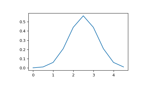
>>> import matplotlib.pyplot as plt
>>> from scipy.stats import multivariate_normal

>>> x = np.linspace(0, 5, 10, endpoint=False)
>>> y = multivariate_normal.pdf(x, mean=2.5, cov=0.5); y
array([ 0.00108914,  0.01033349,  0.05946514,  0.20755375,  0.43939129,
        0.56418958,  0.43939129,  0.20755375,  0.05946514,  0.01033349])
>>> fig1 = plt.figure()
>>> ax = fig1.add_subplot(111)
>>> ax.plot(x, y)

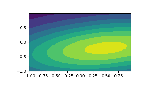
The input quantiles can be any shape of array, as long as the last axis labels the components. This allows us for instance to display the frozen pdf for a non-isotropic random variable in 2D as follows:

>>> x, y = np.mgrid[-1:1:.01, -1:1:.01]
>>> pos = np.dstack((x, y))
>>> rv = multivariate_normal([0.5, -0.2], [[2.0, 0.3], [0.3, 0.5]])
>>> fig2 = plt.figure()
>>> ax2 = fig2.add_subplot(111)
>>> ax2.contourf(x, y, rv.pdf(pos))

Methods

``pdf(x, mean=None, cov=1, allow_singular=False)``	Probability density function.
``logpdf(x, mean=None, cov=1, allow_singular=False)``	Log of the probability density function.
``cdf(x, mean=None, cov=1, allow_singular=False, maxpts=1000000*dim, abseps=1e-5, releps=1e-5)``	Cumulative distribution function.
``logcdf(x, mean=None, cov=1, allow_singular=False, maxpts=1000000*dim, abseps=1e-5, releps=1e-5)``	Log of the cumulative distribution function.
``rvs(mean=None, cov=1, size=1, random_state=None)``	Draw random samples from a multivariate normal distribution.
``entropy()``	Compute the differential entropy of the multivariate normal.