scipy.signal.lsim2
-
scipy.signal.lsim2(system, U=None, T=None, X0=None, **kwargs)[source]¶ Simulate output of a continuous-time linear system, by using the ODE solver
scipy.integrate.odeint.- Parameters
- systeman instance of the
lticlass or a tuple describing the system. The following gives the number of elements in the tuple and the interpretation:
1: (instance of
lti)2: (num, den)
3: (zeros, poles, gain)
4: (A, B, C, D)
- Uarray_like (1D or 2D), optional
An input array describing the input at each time T. Linear interpolation is used between given times. If there are multiple inputs, then each column of the rank-2 array represents an input. If U is not given, the input is assumed to be zero.
- Tarray_like (1D or 2D), optional
The time steps at which the input is defined and at which the output is desired. The default is 101 evenly spaced points on the interval [0,10.0].
- X0array_like (1D), optional
The initial condition of the state vector. If X0 is not given, the initial conditions are assumed to be 0.
- kwargsdict
Additional keyword arguments are passed on to the function odeint. See the notes below for more details.
- systeman instance of the
- Returns
- T1D ndarray
The time values for the output.
- youtndarray
The response of the system.
- xoutndarray
The time-evolution of the state-vector.
See also
Notes
This function uses
scipy.integrate.odeintto solve the system’s differential equations. Additional keyword arguments given tolsim2are passed on to odeint. See the documentation forscipy.integrate.odeintfor the full list of arguments.If (num, den) is passed in for
system, coefficients for both the numerator and denominator should be specified in descending exponent order (e.g.s^2 + 3s + 5would be represented as[1, 3, 5]).Examples
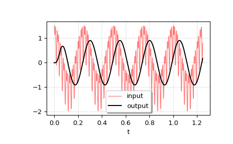
We’ll use
lsim2to simulate an analog Bessel filter applied to a signal.>>> from scipy.signal import bessel, lsim2 >>> import matplotlib.pyplot as plt
Create a low-pass Bessel filter with a cutoff of 12 Hz.
>>> b, a = bessel(N=5, Wn=2*np.pi*12, btype='lowpass', analog=True)
Generate data to which the filter is applied.
>>> t = np.linspace(0, 1.25, 500, endpoint=False)
The input signal is the sum of three sinusoidal curves, with frequencies 4 Hz, 40 Hz, and 80 Hz. The filter should mostly eliminate the 40 Hz and 80 Hz components, leaving just the 4 Hz signal.
>>> u = (np.cos(2*np.pi*4*t) + 0.6*np.sin(2*np.pi*40*t) +
...      0.5*np.cos(2*np.pi*80*t))
Simulate the filter with
lsim2.>>> tout, yout, xout = lsim2((b, a), U=u, T=t)
Plot the result.
>>> plt.plot(t, u, 'r', alpha=0.5, linewidth=1, label='input')
>>> plt.plot(tout, yout, 'k', linewidth=1.5, label='output')
>>> plt.legend(loc='best', shadow=True, framealpha=1)
>>> plt.grid(alpha=0.3)
>>> plt.xlabel('t')
>>> plt.show()
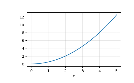
In a second example, we simulate a double integrator
y'' = u, with a constant inputu = 1. We’ll use the state space representation of the integrator.>>> from scipy.signal import lti >>> A = np.array([[0, 1], [0, 0]]) >>> B = np.array([[0], [1]]) >>> C = np.array([[1, 0]]) >>> D = 0 >>> system = lti(A, B, C, D)
t and u define the time and input signal for the system to be simulated.
>>> t = np.linspace(0, 5, num=50)
>>> u = np.ones_like(t)
Compute the simulation, and then plot y. As expected, the plot shows the curve
y = 0.5*t**2.>>> tout, y, x = lsim2(system, u, t) >>> plt.plot(t, y) >>> plt.grid(alpha=0.3) >>> plt.xlabel('t') >>> plt.show()