scipy.optimize.root#

scipy.optimize.root(fun, x0, args=(), method='hybr', jac=None, tol=None, callback=None, options=None)[source]#

Find a root of a vector function.

Parameters:

funcallable

A vector function to find a root of.

x0ndarray

Initial guess.

argstuple, optional

Extra arguments passed to the objective function and its Jacobian.

methodstr, optional

Type of solver. Should be one of

‘hybr’ (see here)

‘lm’ (see here)

‘broyden1’ (see here)

‘broyden2’ (see here)

‘anderson’ (see here)

‘linearmixing’ (see here)

‘diagbroyden’ (see here)

‘excitingmixing’ (see here)

‘krylov’ (see here)

‘df-sane’ (see here)

jacbool or callable, optional

If jac is a Boolean and is True, fun is assumed to return the value of Jacobian along with the objective function. If False, the Jacobian will be estimated numerically. jac can also be a callable returning the Jacobian of fun. In this case, it must accept the same arguments as fun.

tolfloat, optional

Tolerance for termination. For detailed control, use solver-specific options.

callbackfunction, optional

Optional callback function. It is called on every iteration as callback(x, f) where x is the current solution and f the corresponding residual. For all methods but ‘hybr’ and ‘lm’.

optionsdict, optional

A dictionary of solver options. E.g., xtol or maxiter, see show_options() for details.

Returns:

solOptimizeResult: The solution represented as a OptimizeResult object. Important attributes are: x the solution array, success a Boolean flag indicating if the algorithm exited successfully and message which describes the cause of the termination. See OptimizeResult for a description of other attributes.

See also

show_options: Additional options accepted by the solvers

Notes

This section describes the available solvers that can be selected by the ‘method’ parameter. The default method is hybr.

Method hybr uses a modification of the Powell hybrid method as implemented in MINPACK [1].

Method lm solves the system of nonlinear equations in a least squares sense using a modification of the Levenberg-Marquardt algorithm as implemented in MINPACK [1].

Method df-sane is a derivative-free spectral method. [3]

Methods broyden1, broyden2, anderson, linearmixing, diagbroyden, excitingmixing, krylov are inexact Newton methods, with backtracking or full line searches [2]. Each method corresponds to a particular Jacobian approximations.

Method broyden1 uses Broyden’s first Jacobian approximation, it is known as Broyden’s good method.
Method broyden2 uses Broyden’s second Jacobian approximation, it is known as Broyden’s bad method.
Method anderson uses (extended) Anderson mixing.
Method Krylov uses Krylov approximation for inverse Jacobian. It is suitable for large-scale problem.
Method diagbroyden uses diagonal Broyden Jacobian approximation.
Method linearmixing uses a scalar Jacobian approximation.
Method excitingmixing uses a tuned diagonal Jacobian approximation.

Warning

The algorithms implemented for methods diagbroyden, linearmixing and excitingmixing may be useful for specific problems, but whether they will work may depend strongly on the problem.

Added in version 0.11.0.

References

[1] (1,2)

More, Jorge J., Burton S. Garbow, and Kenneth E. Hillstrom. 1980. User Guide for MINPACK-1.

[2]

C. T. Kelley. 1995. Iterative Methods for Linear and Nonlinear Equations. Society for Industrial and Applied Mathematics. <https://archive.siam.org/books/kelley/fr16/>

[3]

La Cruz, J.M. Martinez, M. Raydan. Math. Comp. 75, 1429 (2006).

Examples

The following functions define a system of nonlinear equations and its jacobian.

>>> import numpy as np
>>> def fun(x):
...     return [x[0]  + 0.5 * (x[0] - x[1])**3 - 1.0,
...             0.5 * (x[1] - x[0])**3 + x[1]]

>>> def jac(x):
...     return np.array([[1 + 1.5 * (x[0] - x[1])**2,
...                       -1.5 * (x[0] - x[1])**2],
...                      [-1.5 * (x[1] - x[0])**2,
...                       1 + 1.5 * (x[1] - x[0])**2]])

A solution can be obtained as follows.

>>> from scipy import optimize
>>> sol = optimize.root(fun, [0, 0], jac=jac, method='hybr')
>>> sol.x
array([ 0.8411639,  0.1588361])

Large problem

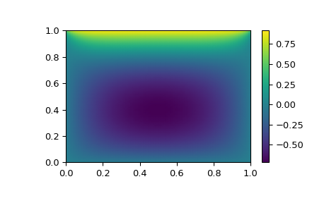
Suppose that we needed to solve the following integrodifferential equation on the square \([0,1]\times[0,1]\):

\[\nabla^2 P = 10 \left(\int_0^1\int_0^1\cosh(P)\,dx\,dy\right)^2\]

with \(P(x,1) = 1\) and \(P=0\) elsewhere on the boundary of the square.

The solution can be found using the method='krylov' solver:

>>> from scipy import optimize
>>> # parameters
>>> nx, ny = 75, 75
>>> hx, hy = 1./(nx-1), 1./(ny-1)

>>> P_left, P_right = 0, 0
>>> P_top, P_bottom = 1, 0

>>> def residual(P):
...    d2x = np.zeros_like(P)
...    d2y = np.zeros_like(P)
...
...    d2x[1:-1] = (P[2:]   - 2*P[1:-1] + P[:-2]) / hx/hx
...    d2x[0]    = (P[1]    - 2*P[0]    + P_left)/hx/hx
...    d2x[-1]   = (P_right - 2*P[-1]   + P[-2])/hx/hx
...
...    d2y[:,1:-1] = (P[:,2:] - 2*P[:,1:-1] + P[:,:-2])/hy/hy
...    d2y[:,0]    = (P[:,1]  - 2*P[:,0]    + P_bottom)/hy/hy
...    d2y[:,-1]   = (P_top   - 2*P[:,-1]   + P[:,-2])/hy/hy
...
...    return d2x + d2y - 10*np.cosh(P).mean()**2

>>> guess = np.zeros((nx, ny), float)
>>> sol = optimize.root(residual, guess, method='krylov')
>>> print('Residual: %g' % abs(residual(sol.x)).max())
Residual: 5.7972e-06  # may vary

>>> import matplotlib.pyplot as plt
>>> x, y = np.mgrid[0:1:(nx*1j), 0:1:(ny*1j)]
>>> plt.pcolormesh(x, y, sol.x, shading='gouraud')
>>> plt.colorbar()
>>> plt.show()