scipy.special.iv#
- scipy.special.iv(v, z, out=None) = <ufunc 'iv'>#
Modified Bessel function of the first kind of real order.
- Parameters:
- varray_like
Order. If z is of real type and negative, v must be integer valued.
- zarray_like of float or complex
Argument.
- outndarray, optional
Optional output array for the function values
- Returns:
- scalar or ndarray
Values of the modified Bessel function.
See also
Notes
For real z and \(v \in [-50, 50]\), the evaluation is carried out using Temme’s method [1]. For larger orders, uniform asymptotic expansions are applied.
For complex z and positive v, the AMOS [2] zbesi routine is called. It uses a power series for small z, the asymptotic expansion for large abs(z), the Miller algorithm normalized by the Wronskian and a Neumann series for intermediate magnitudes, and the uniform asymptotic expansions for \(I_v(z)\) and \(J_v(z)\) for large orders. Backward recurrence is used to generate sequences or reduce orders when necessary.
The calculations above are done in the right half plane and continued into the left half plane by the formula,
\[I_v(z \exp(\pm\imath\pi)) = \exp(\pm\pi v) I_v(z)\](valid when the real part of z is positive). For negative v, the formula
\[I_{-v}(z) = I_v(z) + \frac{2}{\pi} \sin(\pi v) K_v(z)\]is used, where \(K_v(z)\) is the modified Bessel function of the second kind, evaluated using the AMOS routine zbesk.
References
[1]Temme, Journal of Computational Physics, vol 21, 343 (1976)
[2]Donald E. Amos, “AMOS, A Portable Package for Bessel Functions of a Complex Argument and Nonnegative Order”, http://netlib.org/amos/
Examples
Evaluate the function of order 0 at one point.
>>> from scipy.special import iv
>>> iv(0, 1.)
1.2660658777520084
Evaluate the function at one point for different orders.
>>> iv(0, 1.), iv(1, 1.), iv(1.5, 1.)
(1.2660658777520084, 0.565159103992485, 0.2935253263474798)
The evaluation for different orders can be carried out in one call by providing a list or NumPy array as argument for the v parameter:
>>> iv([0, 1, 1.5], 1.)
array([1.26606588, 0.5651591 , 0.29352533])
Evaluate the function at several points for order 0 by providing an array for z.
>>> import numpy as np
>>> points = np.array([-2., 0., 3.])
>>> iv(0, points)
array([2.2795853 , 1.        , 4.88079259])
If z is an array, the order parameter v must be broadcastable to the correct shape if different orders shall be computed in one call. To calculate the orders 0 and 1 for an 1D array:
>>> orders = np.array([[0], [1]])
>>> orders.shape
(2, 1)
>>> iv(orders, points)
array([[ 2.2795853 ,  1.        ,  4.88079259],
       [-1.59063685,  0.        ,  3.95337022]])
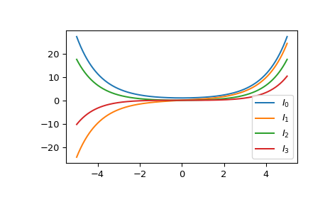
Plot the functions of order 0 to 3 from -5 to 5.
>>> import matplotlib.pyplot as plt
>>> fig, ax = plt.subplots()
>>> x = np.linspace(-5., 5., 1000)
>>> for i in range(4):
...     ax.plot(x, iv(i, x), label=f'$I_{i!r}$')
>>> ax.legend()
>>> plt.show()
