scipy.signal.csd#

scipy.signal.csd(x, y, fs=1.0, window='hann', nperseg=None, noverlap=None, nfft=None, detrend='constant', return_onesided=True, scaling='density', axis=-1, average='mean')[source]#

Estimate the cross power spectral density, Pxy, using Welch’s method.

Parameters:

xarray_like: Time series of measurement values
yarray_like: Time series of measurement values
fsfloat, optional: Sampling frequency of the x and y time series. Defaults to 1.0.
windowstr or tuple or array_like, optional: Desired window to use. If window is a string or tuple, it is passed to get_window to generate the window values, which are DFT-even by default. See get_window for a list of windows and required parameters. If window is array_like it will be used directly as the window and its length must be nperseg. Defaults to a Hann window.
npersegint, optional: Length of each segment. Defaults to None, but if window is str or tuple, is set to 256, and if window is array_like, is set to the length of the window.
noverlap: int, optional: Number of points to overlap between segments. If None, noverlap = nperseg // 2. Defaults to None.
nfftint, optional: Length of the FFT used, if a zero padded FFT is desired. If None, the FFT length is nperseg. Defaults to None.
detrendstr or function or False, optional: Specifies how to detrend each segment. If detrend is a string, it is passed as the type argument to the detrend function. If it is a function, it takes a segment and returns a detrended segment. If detrend is False, no detrending is done. Defaults to ‘constant’.
return_onesidedbool, optional: If True, return a one-sided spectrum for real data. If False return a two-sided spectrum. Defaults to True, but for complex data, a two-sided spectrum is always returned.
scaling{ ‘density’, ‘spectrum’ }, optional: Selects between computing the cross spectral density (‘density’) where Pxy has units of V**2/Hz and computing the cross spectrum (‘spectrum’) where Pxy has units of V**2, if x and y are measured in V and fs is measured in Hz. Defaults to ‘density’
axisint, optional: Axis along which the CSD is computed for both inputs; the default is over the last axis (i.e. axis=-1).
average{ ‘mean’, ‘median’ }, optional: Method to use when averaging periodograms. If the spectrum is complex, the average is computed separately for the real and imaginary parts. Defaults to ‘mean’.

New in version 1.2.0.

Returns:

fndarray: Array of sample frequencies.
Pxyndarray: Cross spectral density or cross power spectrum of x,y.

See also

periodogram: Simple, optionally modified periodogram
lombscargle: Lomb-Scargle periodogram for unevenly sampled data
welch: Power spectral density by Welch’s method. [Equivalent to csd(x,x)]
coherence: Magnitude squared coherence by Welch’s method.

Notes

By convention, Pxy is computed with the conjugate FFT of X multiplied by the FFT of Y.

If the input series differ in length, the shorter series will be zero-padded to match.

An appropriate amount of overlap will depend on the choice of window and on your requirements. For the default Hann window an overlap of 50% is a reasonable trade off between accurately estimating the signal power, while not over counting any of the data. Narrower windows may require a larger overlap.

Consult the Spectral Analysis section of the SciPy User Guide for a discussion of the scalings of a spectral density and an (amplitude) spectrum.

New in version 0.16.0.

References

[1]

P. Welch, “The use of the fast Fourier transform for the estimation of power spectra: A method based on time averaging over short, modified periodograms”, IEEE Trans. Audio Electroacoust. vol. 15, pp. 70-73, 1967.

[2]

Rabiner, Lawrence R., and B. Gold. “Theory and Application of Digital Signal Processing” Prentice-Hall, pp. 414-419, 1975

Examples

>>> import numpy as np
>>> from scipy import signal
>>> import matplotlib.pyplot as plt
>>> rng = np.random.default_rng()

Generate two test signals with some common features.

>>> fs = 10e3
>>> N = 1e5
>>> amp = 20
>>> freq = 1234.0
>>> noise_power = 0.001 * fs / 2
>>> time = np.arange(N) / fs
>>> b, a = signal.butter(2, 0.25, 'low')
>>> x = rng.normal(scale=np.sqrt(noise_power), size=time.shape)
>>> y = signal.lfilter(b, a, x)
>>> x += amp*np.sin(2*np.pi*freq*time)
>>> y += rng.normal(scale=0.1*np.sqrt(noise_power), size=time.shape)

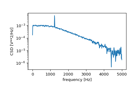
Compute and plot the magnitude of the cross spectral density.

>>> f, Pxy = signal.csd(x, y, fs, nperseg=1024)
>>> plt.semilogy(f, np.abs(Pxy))
>>> plt.xlabel('frequency [Hz]')
>>> plt.ylabel('CSD [V**2/Hz]')
>>> plt.show()