scipy.stats.fligner

scipy.stats.fligner(*samples, center='median', proportiontocut=0.05)

Perform Fligner-Killeen test for equality of variance.

Fligner’s test tests the null hypothesis that all input samples are from populations with equal variances. Fligner-Killeen’s test is distribution free when populations are identical [2].

Parameters:

sample1, sample2, …array_like

Arrays of sample data. Need not be the same length.

center{‘mean’, ‘median’, ‘trimmed’}, optional

Keyword argument controlling which function of the data is used in computing the test statistic. The default is ‘median’.

proportiontocutfloat, optional

When center is ‘trimmed’, this gives the proportion of data points to cut from each end. (See scipy.stats.trim_mean.) Default is 0.05.

Returns:

statisticfloat

The test statistic.

pvaluefloat

The p-value for the hypothesis test.

See also

bartlett

A parametric test for equality of k variances in normal samples

levene

A robust parametric test for equality of k variances

Notes

As with Levene’s test there are three variants of Fligner’s test that differ by the measure of central tendency used in the test. See levene for more information.

Conover et al. (1981) examine many of the existing parametric and nonparametric tests by extensive simulations and they conclude that the tests proposed by Fligner and Killeen (1976) and Levene (1960) appear to be superior in terms of robustness of departures from normality and power [3].

References

[1]

Park, C. and Lindsay, B. G. (1999). Robust Scale Estimation and Hypothesis Testing based on Quadratic Inference Function. Technical Report #99-03, Center for Likelihood Studies, Pennsylvania State University. https://cecas.clemson.edu/~cspark/cv/paper/qif/draftqif2.pdf

[2]

Fligner, M.A. and Killeen, T.J. (1976). Distribution-free two-sample tests for scale. ‘Journal of the American Statistical Association.’ 71(353), 210-213.

[3]

Park, C. and Lindsay, B. G. (1999). Robust Scale Estimation and Hypothesis Testing based on Quadratic Inference Function. Technical Report #99-03, Center for Likelihood Studies, Pennsylvania State University.

[4]

Conover, W. J., Johnson, M. E. and Johnson M. M. (1981). A comparative study of tests for homogeneity of variances, with applications to the outer continental shelf biding data. Technometrics, 23(4), 351-361.

[5]

C.I. BLISS (1952), The Statistics of Bioassay: With Special Reference to the Vitamins, pp 499-503, DOI:10.1016/C2013-0-12584-6.

[6]

B. Phipson and G. K. Smyth. “Permutation P-values Should Never Be Zero: Calculating Exact P-values When Permutations Are Randomly Drawn.” Statistical Applications in Genetics and Molecular Biology 9.1 (2010).

[7]

Ludbrook, J., & Dudley, H. (1998). Why permutation tests are superior to t and F tests in biomedical research. The American Statistician, 52(2), 127-132.

Examples

In [5], the influence of vitamin C on the tooth growth of guinea pigs was investigated. In a control study, 60 subjects were divided into small dose, medium dose, and large dose groups that received daily doses of 0.5, 1.0 and 2.0 mg of vitamin C, respectively. After 42 days, the tooth growth was measured.

The small_dose, medium_dose, and large_dose arrays below record tooth growth measurements of the three groups in microns.

>>> import numpy as np
>>> small_dose = np.array([
...     4.2, 11.5, 7.3, 5.8, 6.4, 10, 11.2, 11.2, 5.2, 7,
...     15.2, 21.5, 17.6, 9.7, 14.5, 10, 8.2, 9.4, 16.5, 9.7
... ])
>>> medium_dose = np.array([
...     16.5, 16.5, 15.2, 17.3, 22.5, 17.3, 13.6, 14.5, 18.8, 15.5,
...     19.7, 23.3, 23.6, 26.4, 20, 25.2, 25.8, 21.2, 14.5, 27.3
... ])
>>> large_dose = np.array([
...     23.6, 18.5, 33.9, 25.5, 26.4, 32.5, 26.7, 21.5, 23.3, 29.5,
...     25.5, 26.4, 22.4, 24.5, 24.8, 30.9, 26.4, 27.3, 29.4, 23
... ])

The fligner statistic is sensitive to differences in variances between the samples.

>>> from scipy import stats
>>> res = stats.fligner(small_dose, medium_dose, large_dose)
>>> res.statistic
1.3878943408857916

The value of the statistic tends to be high when there is a large difference in variances.

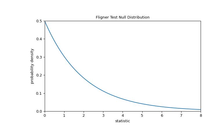
We can test for inequality of variance among the groups by comparing the observed value of the statistic against the null distribution: the distribution of statistic values derived under the null hypothesis that the population variances of the three groups are equal.

For this test, the null distribution follows the chi-square distribution as shown below.

>>> import matplotlib.pyplot as plt
>>> k = 3  # number of samples
>>> dist = stats.chi2(df=k-1)
>>> val = np.linspace(0, 8, 100)
>>> pdf = dist.pdf(val)
>>> fig, ax = plt.subplots(figsize=(8, 5))
>>> def plot(ax):  # we'll re-use this
...     ax.plot(val, pdf, color='C0')
...     ax.set_title("Fligner Test Null Distribution")
...     ax.set_xlabel("statistic")
...     ax.set_ylabel("probability density")
...     ax.set_xlim(0, 8)
...     ax.set_ylim(0, 0.5)
>>> plot(ax)
>>> plt.show()

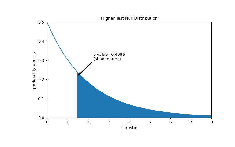
The comparison is quantified by the p-value: the proportion of values in the null distribution greater than or equal to the observed value of the statistic.

>>> fig, ax = plt.subplots(figsize=(8, 5))
>>> plot(ax)
>>> pvalue = dist.sf(res.statistic)
>>> annotation = (f'p-value={pvalue:.4f}\n(shaded area)')
>>> props = dict(facecolor='black', width=1, headwidth=5, headlength=8)
>>> _ = ax.annotate(annotation, (1.5, 0.22), (2.25, 0.3), arrowprops=props)
>>> i = val >= res.statistic
>>> ax.fill_between(val[i], y1=0, y2=pdf[i], color='C0')
>>> plt.show()

>>> res.pvalue
0.49960016501182125

If the p-value is “small” - that is, if there is a low probability of sampling data from distributions with identical variances that produces such an extreme value of the statistic - this may be taken as evidence against the null hypothesis in favor of the alternative: the variances of the groups are not equal. Note that:

• The inverse is not true; that is, the test is not used to provide evidence for the null hypothesis.

• The threshold for values that will be considered “small” is a choice that should be made before the data is analyzed [6] with consideration of the risks of both false positives (incorrectly rejecting the null hypothesis) and false negatives (failure to reject a false null hypothesis).

• Small p-values are not evidence for a large effect; rather, they can only provide evidence for a “significant” effect, meaning that they are unlikely to have occurred under the null hypothesis.

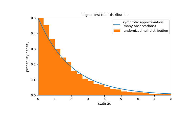
Note that the chi-square distribution provides an asymptotic approximation of the null distribution. For small samples, it may be more appropriate to perform a permutation test: Under the null hypothesis that all three samples were drawn from the same population, each of the measurements is equally likely to have been observed in any of the three samples. Therefore, we can form a randomized null distribution by calculating the statistic under many randomly-generated partitionings of the observations into the three samples.

>>> def statistic(*samples):
...     return stats.fligner(*samples).statistic
>>> ref = stats.permutation_test(
...     (small_dose, medium_dose, large_dose), statistic,
...     permutation_type='independent', alternative='greater'
... )
>>> fig, ax = plt.subplots(figsize=(8, 5))
>>> plot(ax)
>>> bins = np.linspace(0, 8, 25)
>>> ax.hist(
...     ref.null_distribution, bins=bins, density=True, facecolor="C1"
... )
>>> ax.legend(['aymptotic approximation\n(many observations)',
...            'randomized null distribution'])
>>> plot(ax)
>>> plt.show()

>>> ref.pvalue  # randomized test p-value
0.4332  # may vary

Note that there is significant disagreement between the p-value calculated here and the asymptotic approximation returned by fligner above. The statistical inferences that can be drawn rigorously from a permutation test are limited; nonetheless, they may be the preferred approach in many circumstances [7].

Following is another generic example where the null hypothesis would be rejected.

Test whether the lists a, b and c come from populations with equal variances.

>>> a = [8.88, 9.12, 9.04, 8.98, 9.00, 9.08, 9.01, 8.85, 9.06, 8.99]
>>> b = [8.88, 8.95, 9.29, 9.44, 9.15, 9.58, 8.36, 9.18, 8.67, 9.05]
>>> c = [8.95, 9.12, 8.95, 8.85, 9.03, 8.84, 9.07, 8.98, 8.86, 8.98]
>>> stat, p = stats.fligner(a, b, c)
>>> p
0.00450826080004775

The small p-value suggests that the populations do not have equal variances.

This is not surprising, given that the sample variance of b is much larger than that of a and c:

>>> [np.var(x, ddof=1) for x in [a, b, c]]
[0.007054444444444413, 0.13073888888888888, 0.008890000000000002]