scipy.stats.truncnorm

scipy.stats.truncnorm = <scipy.stats._continuous_distns.truncnorm_gen object>

A truncated normal continuous random variable.

As an instance of the rv_continuous class, truncnorm object inherits from it a collection of generic methods (see below for the full list), and completes them with details specific for this particular distribution.

Notes

This distribution is the normal distribution centered on loc (default 0), with standard deviation scale (default 1), and clipped at a, b standard deviations to the left, right (respectively) from loc. If myclip_a and myclip_b are clip values in the sample space (as opposed to the number of standard deviations) then they can be converted to the required form according to:

a, b = (myclip_a - loc) / scale, (myclip_b - loc) / scale

Examples

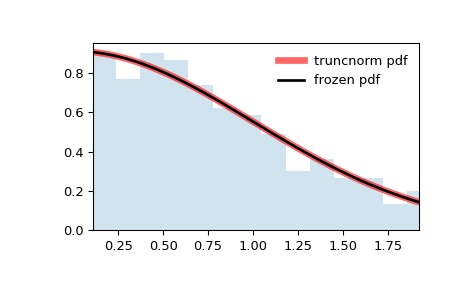
>>> import numpy as np
>>> from scipy.stats import truncnorm
>>> import matplotlib.pyplot as plt
>>> fig, ax = plt.subplots(1, 1)

Calculate the first four moments:

>>> a, b = 0.1, 2
>>> mean, var, skew, kurt = truncnorm.stats(a, b, moments='mvsk')

Display the probability density function (pdf):

>>> x = np.linspace(truncnorm.ppf(0.01, a, b),
...                 truncnorm.ppf(0.99, a, b), 100)
>>> ax.plot(x, truncnorm.pdf(x, a, b),
...        'r-', lw=5, alpha=0.6, label='truncnorm pdf')

Alternatively, the distribution object can be called (as a function) to fix the shape, location and scale parameters. This returns a “frozen” RV object holding the given parameters fixed.

Freeze the distribution and display the frozen pdf:

>>> rv = truncnorm(a, b)
>>> ax.plot(x, rv.pdf(x), 'k-', lw=2, label='frozen pdf')

Check accuracy of cdf and ppf:

>>> vals = truncnorm.ppf([0.001, 0.5, 0.999], a, b)
>>> np.allclose([0.001, 0.5, 0.999], truncnorm.cdf(vals, a, b))
True

Generate random numbers:

>>> r = truncnorm.rvs(a, b, size=1000)

And compare the histogram:

>>> ax.hist(r, density=True, bins='auto', histtype='stepfilled', alpha=0.2)
>>> ax.set_xlim([x[0], x[-1]])
>>> ax.legend(loc='best', frameon=False)
>>> plt.show()

Methods

rvs(a, b, loc=0, scale=1, size=1, random_state=None)	Random variates.
pdf(x, a, b, loc=0, scale=1)	Probability density function.
logpdf(x, a, b, loc=0, scale=1)	Log of the probability density function.
cdf(x, a, b, loc=0, scale=1)	Cumulative distribution function.
logcdf(x, a, b, loc=0, scale=1)	Log of the cumulative distribution function.
sf(x, a, b, loc=0, scale=1)	Survival function (also defined as 1 - cdf, but sf is sometimes more accurate).
logsf(x, a, b, loc=0, scale=1)	Log of the survival function.
ppf(q, a, b, loc=0, scale=1)	Percent point function (inverse of cdf — percentiles).
isf(q, a, b, loc=0, scale=1)	Inverse survival function (inverse of sf).
moment(order, a, b, loc=0, scale=1)	Non-central moment of the specified order.
stats(a, b, loc=0, scale=1, moments=’mv’)	Mean(‘m’), variance(‘v’), skew(‘s’), and/or kurtosis(‘k’).
entropy(a, b, loc=0, scale=1)	(Differential) entropy of the RV.
fit(data)	Parameter estimates for generic data. See scipy.stats.rv_continuous.fit for detailed documentation of the keyword arguments.
expect(func, args=(a, b), loc=0, scale=1, lb=None, ub=None, conditional=False, **kwds)	Expected value of a function (of one argument) with respect to the distribution.
median(a, b, loc=0, scale=1)	Median of the distribution.
mean(a, b, loc=0, scale=1)	Mean of the distribution.
var(a, b, loc=0, scale=1)	Variance of the distribution.
std(a, b, loc=0, scale=1)	Standard deviation of the distribution.
interval(confidence, a, b, loc=0, scale=1)	Confidence interval with equal areas around the median.