scipy.fft.fht#

scipy.fft.fht(a, dln, mu, offset=0.0, bias=0.0)[source]#

Compute the fast Hankel transform.

Computes the discrete Hankel transform of a logarithmically spaced periodic sequence using the FFTLog algorithm [1], [2].

Parameters:

aarray_like (…, n): Real periodic input array, uniformly logarithmically spaced. For multidimensional input, the transform is performed over the last axis.
dlnfloat: Uniform logarithmic spacing of the input array.
mufloat: Order of the Hankel transform, any positive or negative real number.
offsetfloat, optional: Offset of the uniform logarithmic spacing of the output array.
biasfloat, optional: Exponent of power law bias, any positive or negative real number.

Returns:

Aarray_like (…, n): The transformed output array, which is real, periodic, uniformly logarithmically spaced, and of the same shape as the input array.

See also

ifht: The inverse of fht.
fhtoffset: Return an optimal offset for fht.

Notes

This function computes a discrete version of the Hankel transform

\[A(k) = \int_{0}^{\infty} \! a(r) \, J_\mu(kr) \, k \, dr \;,\]

where \(J_\mu\) is the Bessel function of order \(\mu\). The index \(\mu\) may be any real number, positive or negative.

The input array a is a periodic sequence of length \(n\), uniformly logarithmically spaced with spacing dln,

\[a_j = a(r_j) \;, \quad r_j = r_c \exp[(j-j_c) \, \mathtt{dln}]\]

centred about the point \(r_c\). Note that the central index \(j_c = (n-1)/2\) is half-integral if \(n\) is even, so that \(r_c\) falls between two input elements. Similarly, the output array A is a periodic sequence of length \(n\), also uniformly logarithmically spaced with spacing dln

\[A_j = A(k_j) \;, \quad k_j = k_c \exp[(j-j_c) \, \mathtt{dln}]\]

centred about the point \(k_c\).

The centre points \(r_c\) and \(k_c\) of the periodic intervals may be chosen arbitrarily, but it would be usual to choose the product \(k_c r_c = k_j r_{n-1-j} = k_{n-1-j} r_j\) to be unity. This can be changed using the offset parameter, which controls the logarithmic offset \(\log(k_c) = \mathtt{offset} - \log(r_c)\) of the output array. Choosing an optimal value for offset may reduce ringing of the discrete Hankel transform.

If the bias parameter is nonzero, this function computes a discrete version of the biased Hankel transform

\[A(k) = \int_{0}^{\infty} \! a_q(r) \, (kr)^q \, J_\mu(kr) \, k \, dr\]

where \(q\) is the value of bias, and a power law bias \(a_q(r) = a(r) \, (kr)^{-q}\) is applied to the input sequence. Biasing the transform can help approximate the continuous transform of \(a(r)\) if there is a value \(q\) such that \(a_q(r)\) is close to a periodic sequence, in which case the resulting \(A(k)\) will be close to the continuous transform.

References

[1]

Talman J. D., 1978, J. Comp. Phys., 29, 35

[2] (1,2)

Hamilton A. J. S., 2000, MNRAS, 312, 257 (astro-ph/9905191)

Examples

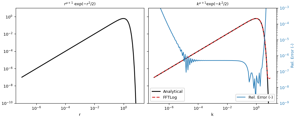
This example is the adapted version of fftlogtest.f which is provided in [2]. It evaluates the integral

\[\int^\infty_0 r^{\mu+1} \exp(-r^2/2) J_\mu(k, r) k dr = k^{\mu+1} \exp(-k^2/2) .\]

>>> import numpy as np
>>> from scipy import fft
>>> import matplotlib.pyplot as plt

Parameters for the transform.

>>> mu = 0.0                     # Order mu of Bessel function
>>> r = np.logspace(-7, 1, 128)  # Input evaluation points
>>> dln = np.log(r[1]/r[0])      # Step size
>>> offset = fft.fhtoffset(dln, initial=-6*np.log(10), mu=mu)
>>> k = np.exp(offset)/r[::-1]   # Output evaluation points

Define the analytical function.

>>> def f(x, mu):
...     """Analytical function: x^(mu+1) exp(-x^2/2)."""
...     return x**(mu + 1)*np.exp(-x**2/2)

Evaluate the function at r and compute the corresponding values at k using FFTLog.

>>> a_r = f(r, mu)
>>> fht = fft.fht(a_r, dln, mu=mu, offset=offset)

For this example we can actually compute the analytical response (which in this case is the same as the input function) for comparison and compute the relative error.

>>> a_k = f(k, mu)
>>> rel_err = abs((fht-a_k)/a_k)

Plot the result.

>>> figargs = {'sharex': True, 'sharey': True, 'constrained_layout': True}
>>> fig, (ax1, ax2) = plt.subplots(1, 2, figsize=(10, 4), **figargs)
>>> ax1.set_title(r'$r^{\mu+1}\ \exp(-r^2/2)$')
>>> ax1.loglog(r, a_r, 'k', lw=2)
>>> ax1.set_xlabel('r')
>>> ax2.set_title(r'$k^{\mu+1} \exp(-k^2/2)$')
>>> ax2.loglog(k, a_k, 'k', lw=2, label='Analytical')
>>> ax2.loglog(k, fht, 'C3--', lw=2, label='FFTLog')
>>> ax2.set_xlabel('k')
>>> ax2.legend(loc=3, framealpha=1)
>>> ax2.set_ylim([1e-10, 1e1])
>>> ax2b = ax2.twinx()
>>> ax2b.loglog(k, rel_err, 'C0', label='Rel. Error (-)')
>>> ax2b.set_ylabel('Rel. Error (-)', color='C0')
>>> ax2b.tick_params(axis='y', labelcolor='C0')
>>> ax2b.legend(loc=4, framealpha=1)
>>> ax2b.set_ylim([1e-9, 1e-3])
>>> plt.show()