scipy.interpolate.splrep
-
scipy.interpolate.splrep(x, y, w=None, xb=None, xe=None, k=3, task=0, s=None, t=None, full_output=0, per=0, quiet=1)[source]¶ Find the B-spline representation of 1-D curve.
Given the set of data points
(x[i], y[i])determine a smooth spline approximation of degree k on the intervalxb <= x <= xe.Parameters: x, y : array_like
The data points defining a curve y = f(x).
w : array_like, optional
Strictly positive rank-1 array of weights the same length as x and y. The weights are used in computing the weighted least-squares spline fit. If the errors in the y values have standard-deviation given by the vector d, then w should be 1/d. Default is ones(len(x)).
xb, xe : float, optional
The interval to fit. If None, these default to x[0] and x[-1] respectively.
k : int, optional
The degree of the spline fit. It is recommended to use cubic splines. Even values of k should be avoided especially with small s values. 1 <= k <= 5
task : {1, 0, -1}, optional
If task==0 find t and c for a given smoothing factor, s.
If task==1 find t and c for another value of the smoothing factor, s. There must have been a previous call with task=0 or task=1 for the same set of data (t will be stored an used internally)
If task=-1 find the weighted least square spline for a given set of knots, t. These should be interior knots as knots on the ends will be added automatically.
s : float, optional
A smoothing condition. The amount of smoothness is determined by satisfying the conditions: sum((w * (y - g))**2,axis=0) <= s where g(x) is the smoothed interpolation of (x,y). The user can use s to control the tradeoff between closeness and smoothness of fit. Larger s means more smoothing while smaller values of s indicate less smoothing. Recommended values of s depend on the weights, w. If the weights represent the inverse of the standard-deviation of y, then a good s value should be found in the range (m-sqrt(2*m),m+sqrt(2*m)) where m is the number of datapoints in x, y, and w. default : s=m-sqrt(2*m) if weights are supplied. s = 0.0 (interpolating) if no weights are supplied.
t : array_like, optional
The knots needed for task=-1. If given then task is automatically set to -1.
full_output : bool, optional
If non-zero, then return optional outputs.
per : bool, optional
If non-zero, data points are considered periodic with period x[m-1] - x[0] and a smooth periodic spline approximation is returned. Values of y[m-1] and w[m-1] are not used.
quiet : bool, optional
Non-zero to suppress messages. This parameter is deprecated; use standard Python warning filters instead.
Returns: tck : tuple
A tuple (t,c,k) containing the vector of knots, the B-spline coefficients, and the degree of the spline.
fp : array, optional
The weighted sum of squared residuals of the spline approximation.
ier : int, optional
An integer flag about splrep success. Success is indicated if ier<=0. If ier in [1,2,3] an error occurred but was not raised. Otherwise an error is raised.
msg : str, optional
A message corresponding to the integer flag, ier.
See also
UnivariateSpline,BivariateSpline,splprep,splev,sproot,spalde,splint,bisplrep,bisplev,BSpline,make_interp_splineNotes
See
splevfor evaluation of the spline and its derivatives. Uses the FORTRAN routinecurfitfrom FITPACK.The user is responsible for assuring that the values of x are unique. Otherwise,
splrepwill not return sensible results.If provided, knots t must satisfy the Schoenberg-Whitney conditions, i.e., there must be a subset of data points
x[j]such thatt[j] < x[j] < t[j+k+1], forj=0, 1,...,n-k-2.This routine zero-pads the coefficients array
cto have the same length as the array of knotst(the trailingk + 1coefficients are ignored by the evaluation routines,splevandBSpline.) This is in contrast withsplprep, which does not zero-pad the coefficients.References
Based on algorithms described in [R113], [R114], [R115], and [R116]:
[R113] (1, 2) P. Dierckx, “An algorithm for smoothing, differentiation and integration of experimental data using spline functions”, J.Comp.Appl.Maths 1 (1975) 165-184. [R114] (1, 2) P. Dierckx, “A fast algorithm for smoothing data on a rectangular grid while using spline functions”, SIAM J.Numer.Anal. 19 (1982) 1286-1304. [R115] (1, 2) P. Dierckx, “An improved algorithm for curve fitting with spline functions”, report tw54, Dept. Computer Science,K.U. Leuven, 1981. [R116] (1, 2) P. Dierckx, “Curve and surface fitting with splines”, Monographs on Numerical Analysis, Oxford University Press, 1993. Examples
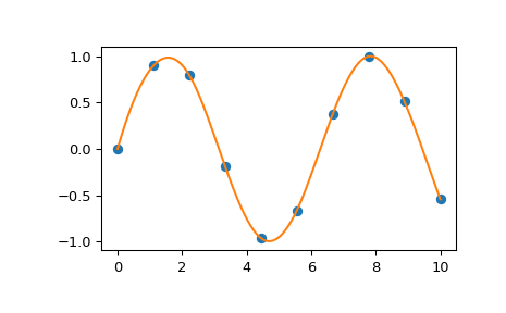
>>> import matplotlib.pyplot as plt
>>> from scipy.interpolate import splev, splrep
>>> x = np.linspace(0, 10, 10)
>>> y = np.sin(x)
>>> spl = splrep(x, y)
>>> x2 = np.linspace(0, 10, 200)
>>> y2 = splev(x2, spl)
>>> plt.plot(x, y, 'o', x2, y2)
>>> plt.show()

