scipy.signal.cheby1

scipy.signal.cheby1(N, rp, Wn, btype='low', analog=False, output='ba')

Chebyshev type I digital and analog filter design.

Design an Nth order digital or analog Chebyshev type I filter and return the filter coefficients in (B,A) or (Z,P,K) form.

Parameters :

N : int

The order of the filter.

rp : float

The maximum ripple allowed below unity gain in the passband. Specified in decibels, as a positive number.

Wn : array_like

A scalar or length-2 sequence giving the critical frequencies. For Type I filters, this is the point in the transition band at which the gain first drops below -rp. For digital filters, Wn is normalized from 0 to 1, where 1 is the Nyquist frequency, pi radians/sample. (Wn is thus in half-cycles / sample.) For analog filters, Wn is an angular frequency (e.g. rad/s).

btype : {‘lowpass’, ‘highpass’, ‘bandpass’, ‘bandstop’}, optional

The type of filter. Default is ‘lowpass’.

analog : bool, optional

When True, return an analog filter, otherwise a digital filter is returned.

output : {‘ba’, ‘zpk’}, optional

Type of output: numerator/denominator (‘ba’) or pole-zero (‘zpk’). Default is ‘ba’.

Returns :

b, a : ndarray, ndarray

Numerator (b) and denominator (a) polynomials of the IIR filter. Only returned if output='ba'.

z, p, k : ndarray, ndarray, float

Zeros, poles, and system gain of the IIR filter transfer function. Only returned if output='zpk'.

See also

cheb1ord

Notes

The Chebyshev type I filter maximizes the rate of cutoff between the frequency response’s passband and stopband, at the expense of ripple in the passband and increased ringing in the step response.

Type I filters roll off faster than Type II (cheby2), but Type II filters do not have any ripple in the passband.

Examples

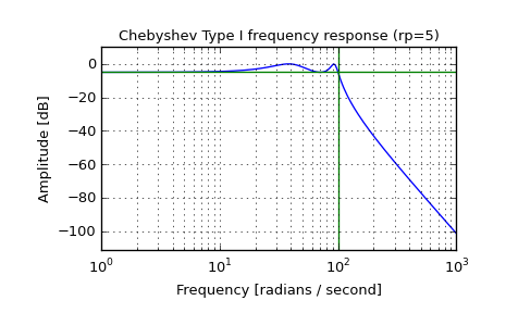
Plot the filter’s frequency response, showing the critical points:

>>> from scipy import signal
>>> import matplotlib.pyplot as plt

>>> b, a = signal.cheby1(4, 5, 100, 'low', analog=True)
>>> w, h = signal.freqs(b, a)
>>> plt.plot(w, 20 * np.log10(abs(h)))
>>> plt.xscale('log')
>>> plt.title('Chebyshev Type I frequency response (rp=5)')
>>> plt.xlabel('Frequency [radians / second]')
>>> plt.ylabel('Amplitude [dB]')
>>> plt.margins(0, 0.1)
>>> plt.grid(which='both', axis='both')
>>> plt.axvline(100, color='green') # cutoff frequency
>>> plt.axhline(-5, color='green') # rp
>>> plt.show()

(Source code)