This is documentation for an old release of SciPy (version 0.12.0). Read this page Search for this page in the documentation of the latest stable release (version 1.15.1).

scipy.signal.freqs

scipy.signal.freqs(b, a, worN=None, plot=None)

Compute frequency response of analog filter.

Given the numerator b and denominator a of a filter, compute its frequency response:

        b[0]*(jw)**(nb-1) + b[1]*(jw)**(nb-2) + ... + b[nb-1]
H(w) = -------------------------------------------------------
        a[0]*(jw)**(na-1) + a[1]*(jw)**(na-2) + ... + a[na-1]

Parameters :

b : ndarray

Numerator of a linear filter.

a : ndarray

Denominator of a linear filter.

worN : {None, int}, optional

If None, then compute at 200 frequencies around the interesting parts of the response curve (determined by pole-zero locations). If a single integer, then compute at that many frequencies. Otherwise, compute the response at frequencies given in worN.

plot : callable

A callable that takes two arguments. If given, the return parameters w and h are passed to plot. Useful for plotting the frequency response inside freqs.

Returns :

w : ndarray

The frequencies at which h was computed.

h : ndarray

The frequency response.

See also

freqz

Compute the frequency response of a digital filter.

Notes

Using Matplotlib’s “plot” function as the callable for plot produces unexpected results, this plots the real part of the complex transfer function, not the magnitude.

Examples

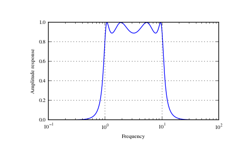
>>> from scipy.signal import freqs, iirfilter

>>> b, a = iirfilter(4, [1, 10], 1, 60, analog=True, ftype='cheby1')

>>> w, h = freqs(b, a, worN=np.logspace(-1, 2, 1000))

>>> import matplotlib.pyplot as plt
>>> plt.semilogx(w, abs(h))
>>> plt.xlabel('Frequency')
>>> plt.ylabel('Amplitude response')
>>> plt.grid()
>>> plt.show()

(Source code)