numpy.ma.polyfit
- numpy.ma.polyfit(x, y, deg, rcond=None, full=False)
Least squares polynomial fit.
Fit a polynomial p(x) = p[0] * x**deg + ... + p[deg] of degree deg to points (x, y). Returns a vector of coefficients p that minimises the squared error.
Parameters : x : array_like, shape (M,)
x-coordinates of the M sample points (x[i], y[i]).
y : array_like, shape (M,) or (M, K)
y-coordinates of the sample points. Several data sets of sample points sharing the same x-coordinates can be fitted at once by passing in a 2D-array that contains one dataset per column.
deg : int
Degree of the fitting polynomial
rcond : float, optional
Relative condition number of the fit. Singular values smaller than this relative to the largest singular value will be ignored. The default value is len(x)*eps, where eps is the relative precision of the float type, about 2e-16 in most cases.
full : bool, optional
Switch determining nature of return value. When it is False (the default) just the coefficients are returned, when True diagnostic information from the singular value decomposition is also returned.
Returns : p : ndarray, shape (M,) or (M, K)
Polynomial coefficients, highest power first. If y was 2-D, the coefficients for k-th data set are in p[:,k].
residuals, rank, singular_values, rcond : present only if full = True
Residuals of the least-squares fit, the effective rank of the scaled Vandermonde coefficient matrix, its singular values, and the specified value of rcond. For more details, see linalg.lstsq.
Warns : RankWarning :
The rank of the coefficient matrix in the least-squares fit is deficient. The warning is only raised if full = False.
The warnings can be turned off by
>>> import warnings
>>> warnings.simplefilter('ignore', np.RankWarning)
See also
- polyval
- Computes polynomial values.
- linalg.lstsq
- Computes a least-squares fit.
- scipy.interpolate.UnivariateSpline
- Computes spline fits.
Notes
Any masked values in x is propagated in y, and vice-versa.
References
[R49] Wikipedia, “Curve fitting”, http://en.wikipedia.org/wiki/Curve_fitting [R50] Wikipedia, “Polynomial interpolation”, http://en.wikipedia.org/wiki/Polynomial_interpolation Examples
>>> x = np.array([0.0, 1.0, 2.0, 3.0,  4.0,  5.0])
>>> y = np.array([0.0, 0.8, 0.9, 0.1, -0.8, -1.0])
>>> z = np.polyfit(x, y, 3)
>>> z
array([ 0.08703704, -0.81349206,  1.69312169, -0.03968254])
It is convenient to use poly1d objects for dealing with polynomials:
>>> p = np.poly1d(z)
>>> p(0.5)
0.6143849206349179
>>> p(3.5)
-0.34732142857143039
>>> p(10)
22.579365079365115
High-order polynomials may oscillate wildly:
>>> p30 = np.poly1d(np.polyfit(x, y, 30))
/... RankWarning: Polyfit may be poorly conditioned...
>>> p30(4)
-0.80000000000000204
>>> p30(5)
-0.99999999999999445
>>> p30(4.5)
-0.10547061179440398
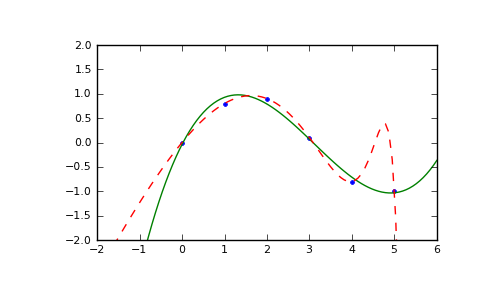
Illustration:
>>> import matplotlib.pyplot as plt
>>> xp = np.linspace(-2, 6, 100)
>>> plt.plot(x, y, '.', xp, p(xp), '-', xp, p30(xp), '--')
[<matplotlib.lines.Line2D object at 0x...>, <matplotlib.lines.Line2D object at 0x...>, <matplotlib.lines.Line2D object at 0x...>]
>>> plt.ylim(-2,2)
(-2, 2)
>>> plt.show()
(Source code, png, pdf)
